Timing Solution Glossary
-Permanent versus Temporary cycles
-Stock Memory (SM) or cycles order
-Forecast Stock Memory (FSM)
-Usage of the correlation coefficient
-Walk Forward Analysis (WFA)
Permanent versus Temporary cycles
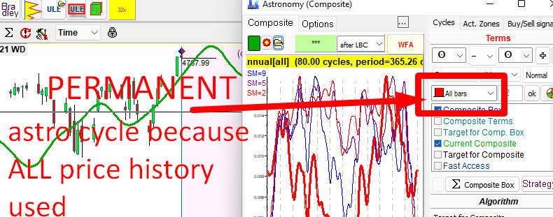
Permanent cycles are the cycles that work in the same manner all the time. So, if we want to deal with the permanent cycle, we will look for a permanent pattern inside the data. In Timing Solution, we can do that in Composite module. To find such pattern, we should use ALL AVAILABLE price history. A good example of permanent cycle is Annual cycle. It works in the same manner all the time: now, in 1950, 1975, 1900, etc. - in any year of the available data.
Here is how the Annual cycle can be done in Composite module. To calculate the Annual cycle shown below, ALL price history is used, this is permanent cycles because we are looking for a permanent Annual pattern:
Permanent cycles are helpful in understanding long-term tendencies on the market. However, we should be careful relying only on these cycles in our trading. We all know by experience that patterns that worked so well for many years may be not that good in a certain year.
That is why the market research moved to Temporary cycles. Temporary cycles also work in the same manner, but for a limited period of time.
Let us build a temporary Annual cycle. We start with the assumption that there is an Annual cycle (we have seen it in Composite module example above). Suppose we want to know how actually this Annual cycle has worked for THE LAST 7 years, not for all available price history. It is quite possible that some permanent pattern is not so strong now. Instead of general outlook of the cycle, we are looking at the latest tendencies in Annual cycle. Do it this way:
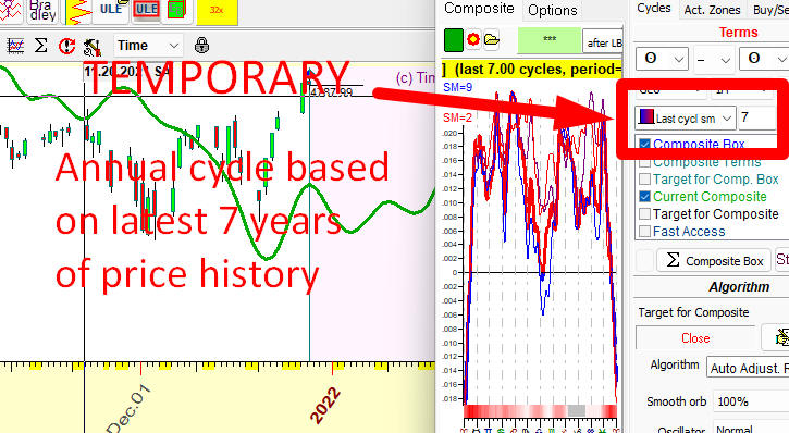
The chart shows how the Annual cycle works for the last 7 years. Clearly, it works a bit differently than in the previous chart: for example, Christmas rally is not so certain now as it used to be.
Similarly we can calculate any temporary astro cycle. Please look at this example of Moon synodic cycle based on the last 12 months (to be precise, 12 full Moon synodic cycles i.e. 12*29.5=354 last days):
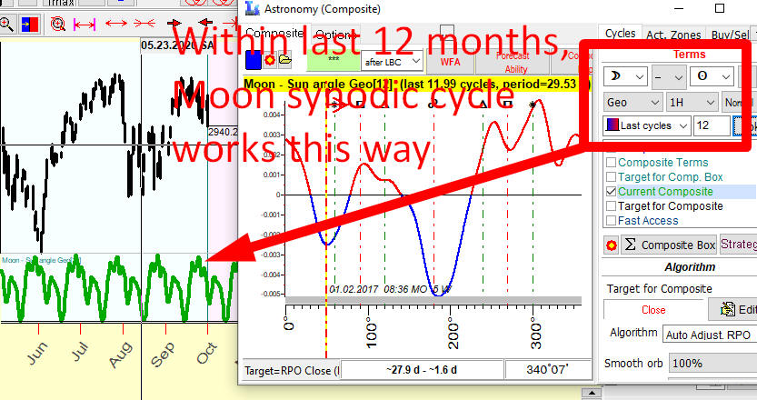
Please pay attention to this parameter, 7 for Annual cycle and 12 for Moon synodic cycle. It is called Stock Memory (SM), and it will be explained later.
There is no fixed, working forever cycles in finance. The only exceptions are cycles used by economists - Kitchen 5 years and Juglar 10-11years cycles. All modules that reveal fixed math cycles (like Spectrum, Q-Spectrum) are oriented to catch temporary cycles. So in all these modules SM parameter is present:

Stock Memory (SM) or cycles order
This is a very important parameter. As I have already mentioned, you can find it in Q-Spectrum, Spectrum and other modules that work with cycles. Here are the examples - in Spectrum, Q-Spectrum, Composite and Trading Spectrum modules:
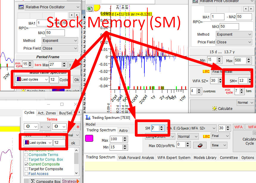
Stock memory (SM) parameter shows how much price history is needed to reveal the presence of some cycle. It indicates a number of periods when cycle manifests itself. As an example, if we analyze 100-days cycle and use SM=12, it means that we use to calculate the importance of this cycle not all available price history, but only its portion: 12x100=1200 days of price history.
We believe that the optimal value is between 5 and 20. Let us consider two extreme cases of too big and too small values of SM:
Case #1. SM is too high: we set SM to 100 and work with the Spectrum module calculating there a periodogram:
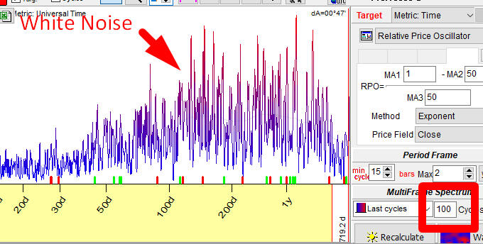
In the statistics it is a situation called "white noise": here all (or almost all) cycles have equal (almost equal) intensity. It is practically impossible to figure out what cycle is less or more important here. We can say with equal assurance that "Anything is working" and "Nothing is working". (To be precise, this is not exactly a white noise, but a gray noise (noise with some structure). Though it does not make a big difference for us.)
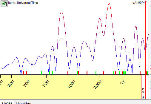
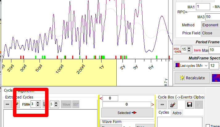
Case #2. SM is too small, we set SM=3 and have calculated a periodogram
with the same Spectrum module. And we have got another face of Chaos:

Now we can see two cycles that could be taken as the most important ones. But - their peaks are too wide here, it may be some cycle with the period between 215 and 250 days. To get a more certain picture we have to apply the bigger value of SM, i.e. use more price history.
Let us set SM=5. The peaks become more narrow, i.e. more certain peaks:
Setting SM=7, we can see two peaks that correspond to 202 and 251 days cycles:
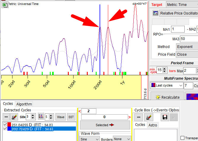
Now we got something to work with.
Also I would like to mention: I tried to find the most correct mathematical entity that describes Stock Memory. From my point of view, the closest one is ORDER in autoregression. It is the amount of past values used in the series to predict the present value. Here is an example: to predict the price today, we used its value yesterday and the day before yesterday; Stock Memory parameter in this case is 2.
Forecast Stock Memory (FSM)
FSM is related to forecast ability of some cycle. It shows how much price history we need to use to get the best forecast based on this cycle. This is not the same as Stock Memory (SM).
Consider the difference between SM and FSM this way: to reveal a cycle, we need to use the last 12 cycles (SM=12), while to get the best forecast based on this cycle we need only the last 5 cycles (FSM=5). The stock memory parameter (SM) is not the same due to the difference of the goals: to find a cycle, the amount of data is important while to get a forecast based on that cycle only the latest price history is relevant.
If you work with Spectrum, you can modify FSM here:
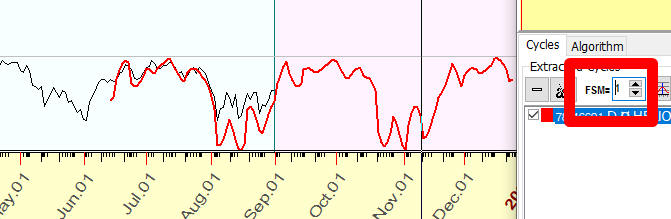
In this example, Spectrum module has revealed a presence of 78 calendar days cycle for S&P500 index (analyzing 12 completed cycles). Then we will try to build a projection line based on that 78-days cycle.
We begin with setting FSM=1, i.e. we try to interpolate the last 78 days of price history with 78-days cycle. As you see, the coincidence is very good:
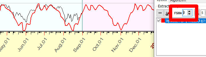
Now we try FSM=2; we try to interpolate the last 2x78=156 days of price history. The coincidence is not that good, though our projection line describes more price history:
And we continue to play with FSM. Please note that when we set FSM=15 (i.e. building a projection line that interpolates last 15 cycles), the projection line describes just major tendencies:
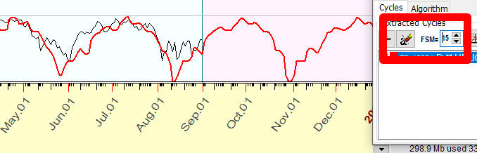
So, changing FSM parameter, we are looking for the balance between over-fitting problem (FSM=1) and too general projection line (FSM=15).
If you work with Q-Spectrum, set FSM here:
Usage of the correlation coefficient
To compare the real price and the projection line, we use a special statistical criterion, named Pearson correlation coefficient. The value of the correlation varies in -1..+1 (-100%..+100%) range.
The value close to +1 (+100%) means that there is a very good coincidence between the real price and the projection line.
Close to 0 (0%) means no coincidence.
Close to -1 (-100%) means inverted coincidence.
In practice we deal with projection lines that provide a correlation at 0.05-0.15, i.e. explain 5%-15% of the price movements.
Here are examples of different projection lines with correlation coefficient values for them:
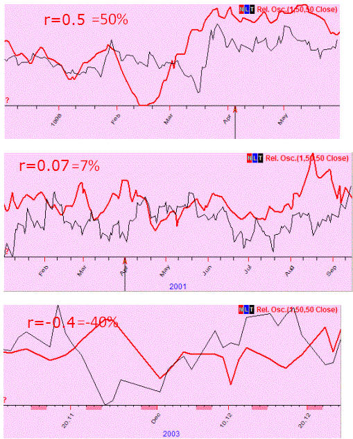
In mathematics, the symbol r is used for correlation. For example, r=0.12 means that the correlation between the price and the projection line is 0.12 (12%).
BUT, in Timing Solution we prefer to show the correlation coefficient as a percentage, like this: r=12%. We do that intentionally. For the first 10 years, we used a classical notation. Later, we have decided to switch to percentage.
The reason is: the typical forecast ability of the projection lines that we built is about 0.1, i.e. 10%. For example, we may have two models; one model provides the correlation r1=0.07, while another has r2=0.007. With "0" and some signs after, it looks confusing. The percentage notation allows to see the result more to the point, not so confusing: r1=7%, r2=0.7%. This is especially important when you browse the list of dozens models with different correlations and need to select only those models that provide the correlation around 0.1 (10%), and higher. The percentage notation is more convenient for this task.
Walk Forward Analysis (WFA)
Non future leaks technology
Today is December 28,2022. Let say, one of your friends
shows the SNP500 forecast for the next year 2023. The forecast is made
with the same model that was used to forecast the same market in the
year 2022. Your friend applied that model for the year 2023 just because
the forecast for the year 2022 worked extremely well... Before doing
anything, ask yourself a simple question: when the forecast for the year
2022 has been done: 1) a year ago
when there was no recorded price history for the year 2022 yet, or 2)
recently, maybe today, with the use of all available price history?
In
the first case we deal with non
future leaks approach: a forecast is made in advance, for
something that is still unknown (the price history for the year 2022 was
not collected then, in the end of 2021). In the second case, it is a post factum forecast,
and this approach
contains future leaks.
WFA one Step
To prevent future leaks, the best way would be to put aside a new forecast (for the year 2023) and wait till December 28, 2023. Only then it will be possible to compare this forecast with the recorded price history, recorded during the year 2023. Only then we will see the real value of this forecast as well of the model used to make it.
Sample Size (SZ)
To understand better how this forecast works (or how well the applied model works), it would be good to repeat this procedure the next year: in December 2023 make a forecast for the year 2024, put this forecast in a safe place for a year and look at it again in December 2024 comparing it to the actual price chart. It would be great to repeat this procedure 10 times at least. So, we would do 10 WFA steps. The amount of WFA steps is called "Sample Size" (SZ). In our example, it would be great to have SZ=10.
Walk Forward Analysis
This approach - looking forward and comparing actual values to the forecasted ones - is good in a sense that there is no future leaks at all. The problem of this approach is: we need to wait for 10 years at least to complete this analysis and make some conclusions. It will be too late for a practical use. In ten years from now, we probably will be able to say that the model used for forecasts for all those years is good. It may turn out being not good at all. This knowledge that we get in 10 years from now - it is useless for us today.
Now, is there anything we could do to ensure that we follow this approach that has no future leaks (and therefore provides a genuine, true forecast) and get some practical value for today's trading?
The answer is - yes. We can put your friend and his/her model used for the forecast in the PAST, 10 years back. How do we do that? Simply cutting the price chart onto pieces. Give your friend the piece of the price chart for SNP500 that ends in December 2012 and ask to make a forecast for the year 2013. Then open the data for the year 2013 and compare with the projection line. Then add to your friend's data this 2013 piece, asking to make a forecast for the next year, which would be 2014. Again, compare it with the recorded data for the year 2014 - and request a forecast for the year 2015. And so on... This way, the information regarding the model's forecast ability will be received, and there will be no future leaks. No need to wait for 10 years to verify the model. You only need to be sure that your friend has no access to the price data that you have today, to prevent any future leaks.
In Timing Solution, this analysis can be done automatically, and we guarantee that there are no future leaks there.
WFA report/chart
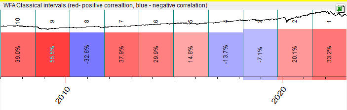
This is how the result of Walk Forward Analysis looks:
Red bars here represent years when the projection line has forecasted the price well; the numbers show the correlation between the price chart and the projection line. Blue bars correspond to the negative correlation between the price and the projection line - forecast either is not working there or works in inverted mode.
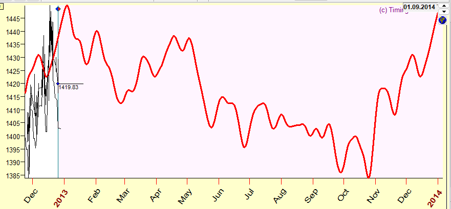
For example, the first bar there (the red one) covers the period of December 2012 - December 2013:
The program makes a forecast using the price history prior December 2012; forecast is made for a period till December 2013. This is non future leaks forecast, as the program does not "know" about the price history after December 2012 (it uses data prior to that; it is achieved by positioning LBC at Dec.28, 2012). When the forecast is done, it is compared to the next portion of data (after LBC), to the actual price in 2013. This is how it looks; this projection line reflects SNP500 movement for year 2013 with the accuracy 29% (r=0.29):
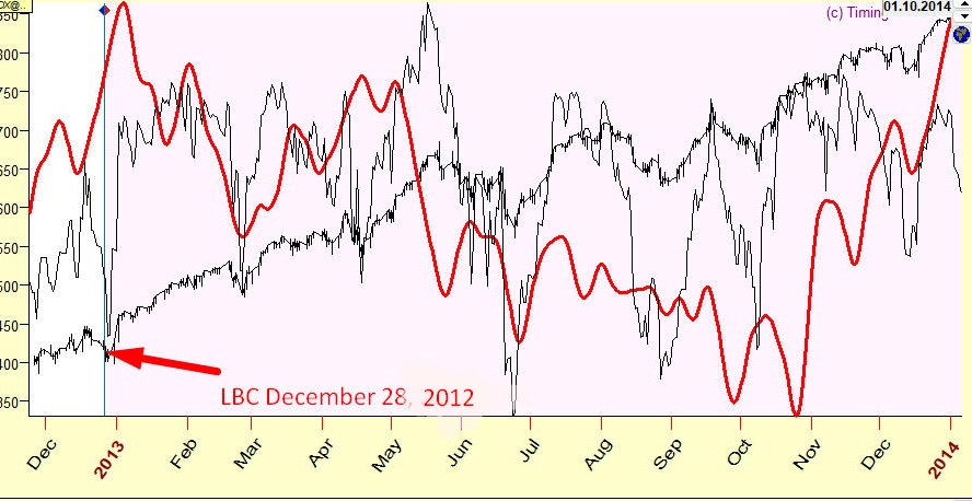
The same procedure is repeated for other years - 2014, 2015 .. 2022.
Avoiding future leaks is the major issue for any forecast. You have to be sure that it is really a forecast, not just the imitation of some previously recorded data set. In other words, the true forecast must be "blind": if, as an example, you make a forecast for the year 2013, you need to be absolutely sure that the actual price for 2013, even a small piece of it, is not used in the process of making that forecast.
How can we be sure that Timing Solution software follows this rule? You can easily check if there are any future leaks there. As an example, let us consider the forecast for the year 2013. Keep the picture above somewhere. Now, make a data file and download SNP500 price history up to December 2012. As you have created the data file yourselves, you know that the price for 2013 is not included there. Therefore, the program, Timing Solution, simply does not "know" about the data in 2013 and cannot work with these data. Using the same model, make a forecast. It will be exactly the same as in the picture above. Here it is:
Making a forecast, we do not have Undo button, it is always final....
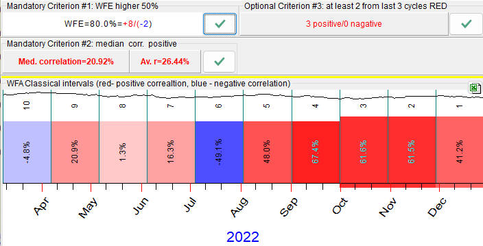
Walk Forward Efficiency (WFE)
In the example above we have totally 6 years with the positive correlation, "good" years when our projection line works properly. Also there are 4 years with the negative correlation, "bad" years when our model does not work or works in inverted mode:
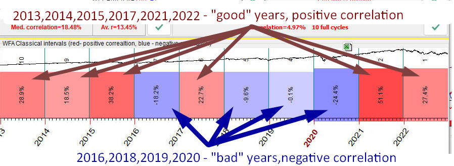
The amount of "good" years with positive correlation is 60% (6 years of the available 10). This value is called Walk Forward Efficiency of the model, or WFE. Obviously the more red (positive correlation) bars the WFA reports has, the higher WFE value is, the better model we have.
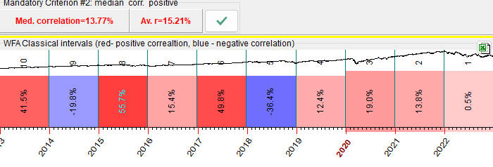
Look at another example of "good" model. Here, for 8 years of 10, the projection line works properly, WFE=80%:
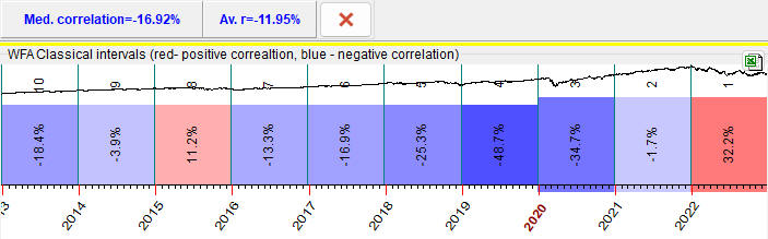
Compare it to this example of "bad" models: there the model works properly only for 2 years of 10; WFE=20%:
It is recommended to choose models that have a maximum amount of red bars, with high WFE value.
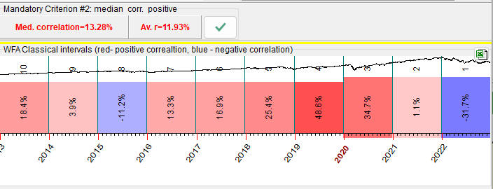
AVR - average and median correlation (varies -100%..+100%)
Also pay attention to median and averaged values of correlation:
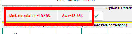
This is another important parameter, the average or median correlation for these 10 (or any other number) testing intervals.
If the median correlation is positive while the average correlation is negative, it means that the model applied can be qualified as a risky model. It works properly for most of the years, though for some years it works completely different, giving the opposite result (possibly inverted).
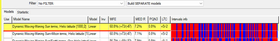
PQN - Projection Quality Number (PQN2 and PQN3) - it is a special parameter that we have developed; it consolidates WFE (walk forward efficiency), AVR (average correlation) and LXC (last X cycles) in one parameter.
There are two versions of PQN:
PQN2 (typically varies in the range -20%..+20%) - consolidates WFE and AVR in one number; the higher total PQN2 means the higher walk forward efficiency and higher average correlation.
PQN3 (typically varies in the
range -20%..+20%) - consolidates WFE and AVR and LXC
parameters in one number. It works the same way as PQN2
parameter plus it also involves last X cycles (L%X). This is a
screenshot from Forecast Mill (FM) library; the models there are
sorted by PQN3:
PQN2 and PQN3 should be positive. If one
of these parameters is negative it indicates a possible
inversion of the projection line.
For example, this
record means:
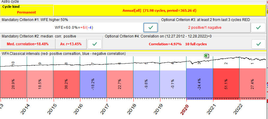
In total, we have analyzed 120 cycles, i.e. vary LBC 120 times, i.e. the sample size=120;
WFE=60.8% (+73/-47) i.e. the correlation between the projection line and the price was positive 73 times versus 47 times when it was negative;
AVR=0.072 (7.2%) i.e. average correlation is 0.072;
L7C=71% (+5/-2) i.e. for the last 7 cycles the correlation was positive 5 times versus 2 time negative;
PQN3 - the projection quality number for this projection line is 0.8%
Typical Period
In the example above we analyzed Annual cycle with the period of one year. Let us try some other cycle, Moon synodic. The period of this cycle is 29.53 days. Accordingly, WFA report looks this way:
One WFA step covers one month of the price history, as we analyze a faster cycle now.
Another one, Venus synodic cycle, has the period of 584 days, so WFA chart looks this way now (one WFA step covers 584 days there):
In other words, we adjust the length of the analyzed interval according to the period of the analyzed cycles.
Inverted Cycles
When we have WFA report like this one:
- most of intervals are blue, negative correlation
- median and average correlations are negative
We may try to treat this cycle as INVERTED one. In Composite module, the option to invert cycle is here:
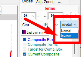
WFA chart for this inverted cycle will look inverted as well:
Warning: Be very cautious with inverted cycles, always try to find first normal/non inverted cycles.
Reading WFA results
Now you should be able to read the output of different modules that conduct Walk Forward Analysis. Here are two examples:
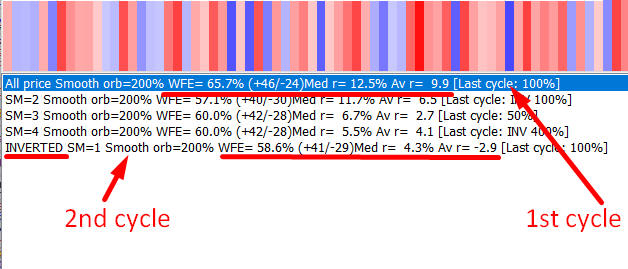
The first cycle shows Walk Forward Efficiency (WFE) 65.7%; 46 intervals there are "good" (positive correlation) versus 24 that are "bad" (negative correlation), median correlation=12.5%, averaged=9.9%
Second cycle works in INVERTED mode, WFE=58.6%, 41 positive versus 29 negative correlation, median correlation=4.3%, average correlation=-2.9%. Median and average correlations have opposite sign hence be careful with this cycle, it maybe risky.