Walk forward analysis of projection lines - definitions
Keywords
Typical period, WFA, Walk forward analysis, LBC - Learning border cursor, Sample size, Correlation, WFE - Walk forward efficiency, AVR - Average correlation, PQN2 PQN3 Projection quality number Forecast horizon, L3C - Last 3 cycles criterion
Here we explain the formal approach that is used for verification of projection lines in Timing Solution software. This approach is based on the classical walk forward analysis that is used in finance to verify trading systems (see Robert Pardo's books). What is new here is a proposed technology of verification of a projection line.
We would like to introduce a kind of a standard to verify any projection line. It means that all modules that incorporate walk forward analysis in Timing Solution are using this approach and are based on these definitions. We think that this standard established once will have no change for the several years.
Let's go.
Suppose we have created some projection line and we need to verify it. Let it be a projection line based on Moon phases cycle.
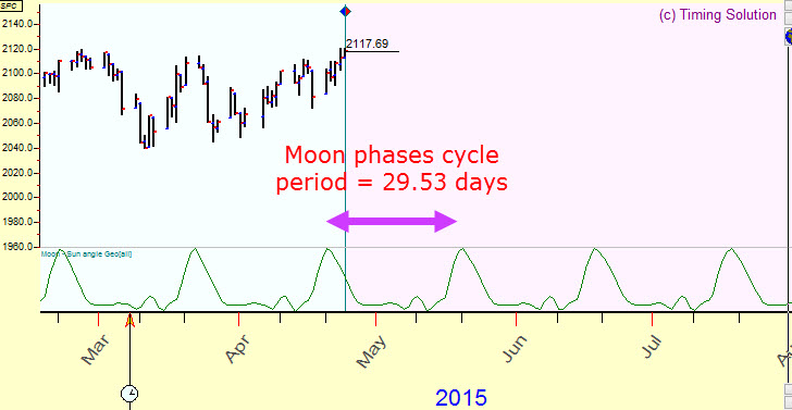
Typical period - this is the first thing you should know, a typical of this projection line. It is a period of the cycle used to create this projection line. In our example, the projection line is based on Moon phases cycle. As we know, the Moon phases cycle represents the cycle between two New Moons. We know as well that the distance between two New Moons is approximately 29.5 days. This value is a period of our cycle.
The picture shows the Moon phases (=synodic) cycle with 29.5 days period:
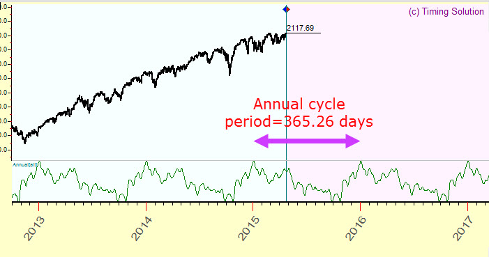
If we would create a projection line based on Annual cycle, it would be a picture of it (Annual cycle with 365.26 days period):
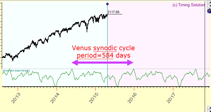
One more example is Venus synodic cycle, with the period of 589 days. Here is how it looks:
One Walk forward analysis step - this is the basis of walk forward analysis. It is a very important issue. Let me explain what it is about. Suppose somebody claims that he/she has developed a projection line for S&P500 based on Moon phases, and he/she wants to demonstrate you how this projection has worked in the past. When you hear that, you better be very careful. What is confusing to me is the words "in the past". Yes, all sciences do make theories based on the facts found in the past. And yes, we can make a projection line based on any idea that it supported with the facts in the past. However, scientists propose some experiments that will confirm or destroy their theories. They do that because they need to be sure that the theory will work in the future. The past is used as a source of ideas, only for that.
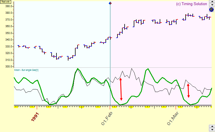
It is applicable to market forecast and market projections. Here is a quick example of the forecast that does not work in reality. Suppose that on February 1, 1991 somebody introduced the model for Moon phases cycle and stressed out how well worked last month (January 1991):
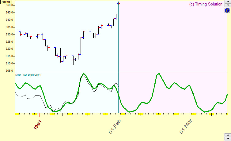
Everything seems OK here: the projection is really based on Moon phases and it really explains price movements since the mid of December 1990 till February 1, 1991. However, this is not a forecast, for a forecast we need something more, some future prospective. If we look at real prices after February 1, 1991 and compare them with this "forecast", here is what we see:
Instead of watching the illustration on how well some projection line was in the past, you may propose this experiment: "Ok, if you think that your projection line worth something, give me a forecast for the next month, and we meet again in one month. Then, having new price history arrived, we will compare your forecast with the real price chart". Obviously this version of the forecast verification looks much more useful than any other. It models a real trader's behavior when the trader has a future forecast and does not have a future price. This is a true "non future leaks technology". We can even improve this technology: we can ask to update monthly forecast in the beginning of each month within one year, and at the end of each month we can compare this forecast with the arrived real price.
If you need to make your opinion about the forecast quickly or you have no time to wait for a year or for a month, you may look at the past data. (The most common situation is: you need to make a decision to buy some product/a service/a software.) However, you must do it in a special way. You must make yourself sure that no future leaks are present.
How this procedure works in Timing Solution?
Here are the New Moon dates for the year 2014:
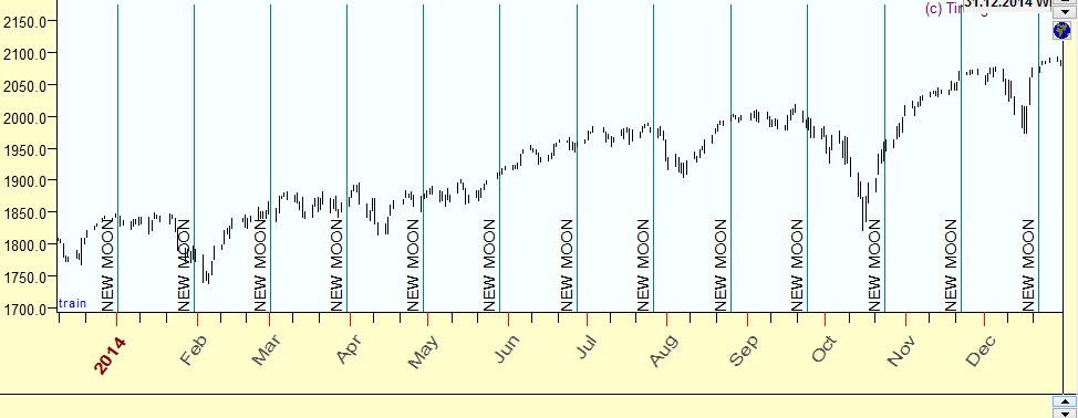
The first New Moon in the year 2014 took place on January 1. Let's use this date (January 1, 2014) as a starting point for our analysis. In other words, we pretend that on January 1, 2014, we ask the program to provide a forecast till January 31, 2014.
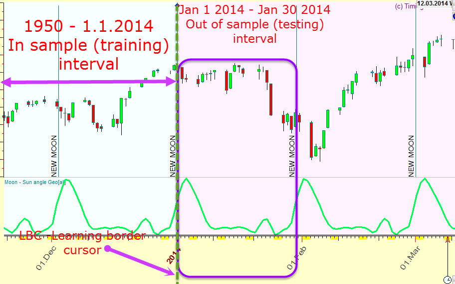
The picture below shows the downloaded S&P500 index price history since the year 1950 up to January 1, 2014, together with its imitation by the model based on Moon phases cycle (the lime curve) and together with the projection line that is a prolongation of that line. This is an important moment: We use the data up to January 1, 2014 to create a line based on Moon phase cycle and we prolong it further. This prolongation is our projection line, we do not use any new price data to create it. After that, we compare how this projection line fits the real price movement within the next synodic Month, i.e. from January 1, 2014 to January 30, 2014. The chart below explains this procedure:
The most important moment is: if you make a forecast that starts on January 1, 2014, you should use for your calculations ONLY the price history prior this date (January 1, 2014). This is a basis of non future leaks technology. We model the behavior of a trader who tries to figure out how this forecast works in advance, not post factum. Once a month he asks to provide a forecast for a month ahead and does that for some period of time.
In other words, in this particular case, when the program calculates a projection line, the price history after January 1, 2014 is totally unknown for the program, it does not affect the calculations. It becomes known when the forecast is made and we want to compare our forecast with the real price after that date, January 1, 2014.
It differs from the situation when a person takes the data up to April 25, 2015 and says: "Look how well my forecast worked for the year 2014, starting from January 1!" What he/she shows you is just the ability of his/her tool to reflect the market moves inside the past data. You should not be surprised if this "forecast" will show nothing close to real market moves after April 25, 2015.
Let's continue to discuss the important definitions.
LBC - Learning Border Cursor: in the example above, the date January 1, 2014 is called Learning Border Cursor (LBC). This is the border between the Past and the Future, between what the program "knows" (i.e. can use for calculations) and "don't know" territory, where the price history is used for the verification of our models only. The portions of the price history used for calculations and the verification should be different and not overlapped. Otherwise we may face the future leaks phenomena. In practice it means that we may create models that describe very well market moves in the past (before LBC) and have one disadvantage - they work good in the past only.
So LBC is the border between what the program "knows" and accordingly what can be used for cooking forecast models and "don't know" territory that tells us the real value of these models. The most misunderstanding in financial modeling happens because "known" and "don't know" data are not separated properly, (we don't know either this is real trade or a fake post factum trade).
In finance mathematics, the price history prior LBC is called in sample price history while after LBC - out of sample. In neural network technology the data prior LBC is called training (optimizing) interval, after LBC - testing interval.
Walk forward analysis procedure- Experienced trader knows very well how his Majesty Chaos may play with us. Some forecast may be very good within one period (29.5 days in this example). It may happen not because of a good model, it could happen accidentally, so that same forecast will fail on the next period. It means that our trader would check this model several times, to have more complete understanding of its forecasting ability.
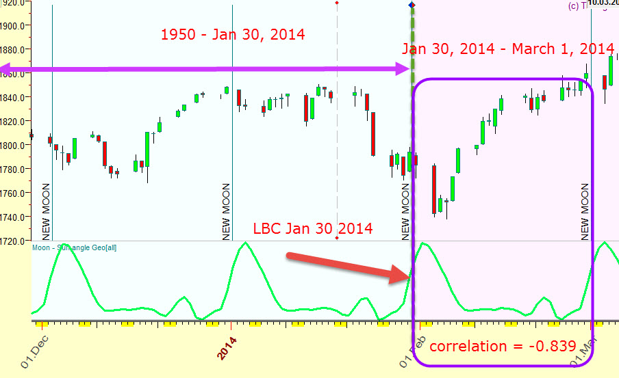
For Moon phases model this procedure works this way: we shift LBC position one period ahead, i.e. 29.5 days ahead, to January 30, 2014. The program calculates the updated projection line (using updated price history up to January 30, 2014) and makes a forecast for one period ahead, since January 30, 2014 till March 1,2014 (out of sample/testing interval):
We compare how this forecast fits real price history on the testing interval and perform this procedure several times. We can monitor this model within a year (12 times) or within 5 years (60 times) or any other.
Sample size- This is amount of LBC shifts, how many times we monitor our models.
One Walk forward analysis step correlation- To compare real price and projection line, we use a special statistical criterion, named Pearson correlation. The value of correlation varies in -1..+1 diapason.
The value close to +1 means that there is a very good coincidence between the real price and the projection line.
Close to 0 means no coincidence.
Close to -1 means inverted coincidence.
In practice we deal with projection lines that provide correlation at 0.05-0.15, i.e. explain 5%-15% of price movements.
Here are examples of different projection lines with correlation coefficient values for them:
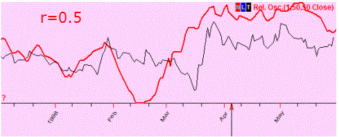
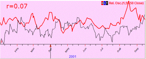
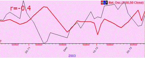
In mathematics, the symbol r is used to designate correlation.
WFE - walk forward efficiency (varies in diapason 0%..100%) - Now we know walk forward analysis procedure: we shift LBC position several times and watch how this projection line works after LBC.
In our example:
#1 walk forward analysis step, LBC 1.1.2104, testing interval 1.1.2014-1.30.2014, the correlation between the price and the projection line on testing interval = 0.235, good coincidence;
#2 walk forward analysis step, LBC 1.30.2104, testing interval 1.30.2014-3.1.2014, the correlation between the price and the projection line on testing interval = -0.839, inversion;
#3 walk forward analysis step, LBC 3.1.2104, testing interval 3.1.2014-3.29.2014, the correlation between the price and the projection line on testing interval = 0.552, good coincidence.
For this example, we have conducted this routine 16 times and received this diagram:
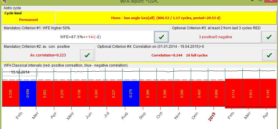
The red/blue bars here represent testing intervals that were used to verification of our model. There are 16 bars there; it means that we have shifted LBC 16 times, i.e. we have asked 16 times to provide a forecast 29.5 days in advance to figure out how our model forecasts the future.
The red bars here correspond to a positive correlation between the price and the projection line, i.e. forecast is good, not inverted at least. The blue bars - negative correlation, i.e. inverted projection line.
This is a very good result: 14 of16 bars are red, i.e. in 87.5% cases we have a good forecast, This parameter is called walk forward efficiency, percentage of red bars, i.e. percentage of good forecasts.
AVR - average correlation (varies in diapason -1..+1)- This is another important parameter, the average correlation for these 16 (or any other number) testing intervals.
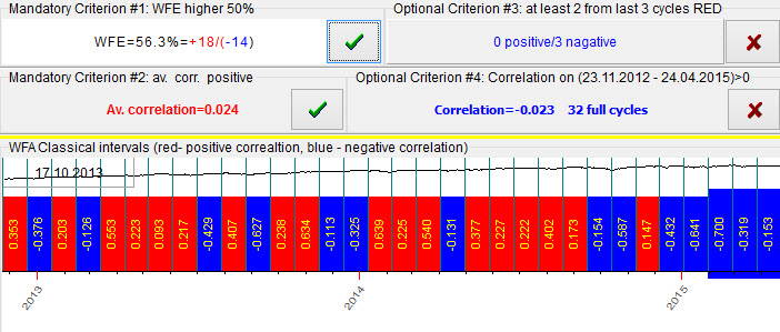
How to choose the cycle We recommend to choose the cycles where these two criteria meet together:
Criterion #1: walk forward efficiency is higher than 50%; i.e. the amount of good forecast (red bars) on the testing interval is bigger than the amount of inverted forecast (blue bars). The higher this value, the more good (not inverted) intervals we have.
Criterion #2: the average correlation for all intervals should be positive. The higher this value, the best fit between the price and the projection line we have.
Forecast horizon - By definition forecast horizon is the interval where this cycle (or projection line) works.
In this class we have analyzed Moon phases cycle. The period of this cycle is 29.5 days, so the forecast horizon for this cycle is also 29.5 days. For Annual cycle with the period of 365.25 days forecast horizon accordingly is 365.25 days. In other words, we recommend to use a typical period of the analyzed cycle as a forecast horizon.
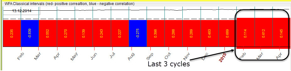
L3C - Last 3 cycles criterion (varies in the range 0%..100%) - There is one more nuance in walk forward analysis. Please look at the picture below. It shows the result of WFA for Moon phases cycle calculated at the end of April 2015:
Let's increase the sample size to 50, i.e. analyze 50 intervals:
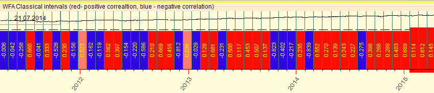
You see, this cycle works well since 2013 though prior to that, in the years
2011-2012, this cycle has worked not so well (there are many blue/inverted
intervals there). So we have to be careful considering how this cycle has worked
RECENTLY. It is possible that it may worked very well earlier and after that it
had stopped to work properly.
This is why we recommend L3C criterion:
watch last three intervals. At least two from those three intervals should be
red, i.e. provide a good forecast. This way we try to prevent a situation when the
cycle generally working good stops working, like in this example:
L4C,L5C,L6C,L7C ... - Last %X cycles criterion (varies in the range 0%..100%) - The same manner we can use more universal criterion that involves last 4,5,6,7.., etc. intervals.
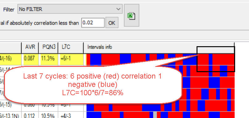
In this report to estimate the performance of our model we use last seven intervals. 6 times correlation was positive while once it was negative. It means that L7C parameter is equal to 100% x 6/7 =86% i.e. for the last seven intervals a correlation is positive in 86% cases.
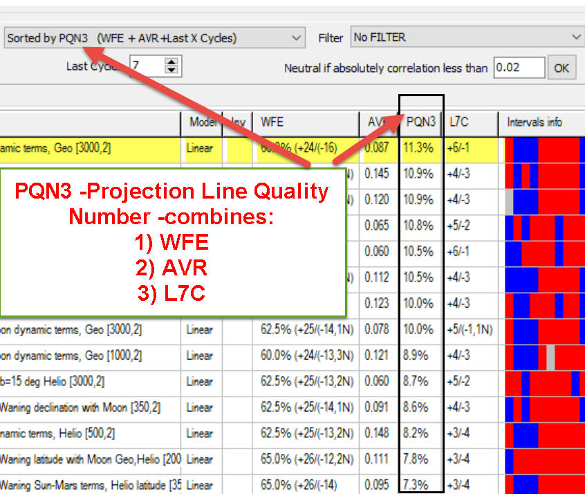
PQN - Projection Quality Number (PQN2 and PQN3) - it is a special parameter that we have developed; it consolidates WFE (walk forward efficiency), AVR (average correlation) and LXC (last X cycles) in one parameter.
There are two versions of PQN:
PQN2 (typically varies in the range -20%..+20%) - consolidates WFE and AVR in one number; the higher total PQN2 means the higher walk forward efficiency and higher average correlation. In practice we recommend to choose the cycles with PQN2 10% and higher.
PQN3 (typically varies in the range -20%..+20%) - consolidates WFE and AVR and LXC parameters in one number. It works the same way as PQN2 parameter plus it also involves last X cycles. This is a screenshot from Forecast Mill (FM) library; the models there are sorted by PQN3:
PQN2 and PQN3 should be positive. If one of these parameters is negative it indicates a possible inversion of the projection line.
For example, this record means:

In total, we have analyzed 40 cycles, i.e. vary LBC 40 times, i.e. the sample size=40;
WFE=66% (+33/-17) i.e. the correlation between the projection line and the price was positive 33 times versus 11 times when it was negative;
AVR=0.090 i.e. average correlation is 0.090;
L7C=86% (+6/-1) i.e. for the last 7 cycles the correlation was positive 6 times versus 1 time negative;
PQN3 - the projection quality number for this projection line is 14.6%