Wild risks, wild randomness
My wife has found this story recently. It was published by Toronto Star newspaper; see it here. This is a story about dramatic results of applying statistics in a not correct way. I would not blame the guy though I would like to discuss the core of this problem.
In a real life, the problem is very simple. It is the problem of evaluation of the risks related to financial data. It is not just an academic exercise; it affects our lives in a very practical sense. As an example, your friend may come to you claiming that he has found one very reliable trading system. He says to you: "It provides 75% winning trades. I have tried it already; it has generated me 100 trading signals, and 75% of them turned be winning ones". What should you do? To figure out how good this system is, normally people imagine such a picture: they toss a coin 100 times, and 75 times they see tails (the analogy of winning trades) while heads (loss) happen only 25 times. If it would be so, this is an extremely reliable result. It leaves no room to casualties, they are practically impossible there. The statistical criteria (chi square) would show that this fact is not casual with the probability 99.95% (chi square=12); in other words, it is not some game of Chaos.
So, it would be really good to have such a system. However, it is not so. It would be true in some ideal world where all timely processes follow the rules of the normal distribution. We live in a real world. In this world, for the last 20 years at least, the most important finding in financial mathematics is the fact that we CANNOT ESTIMATE financial data this way. So forget about tossing the coin when you deal with financial data. Does it mean that the statistics is not working for financial data? Or is it possible that the statistics does not work at all (remember the saying: "There are two kinds of a lie - a simple lie and the statistics")? The answer to both questions is: No. In our real world, we cannot blame statistics and/or mathematics. Mathematicians and statisticians know that dealing with His Majesty Chaos we simply should remember that it has many faces. We just need to know these faces.
Historically, Bachelier was the first one to apply methods of statistics to the stock market (1900). During the next 50 years, the statistics becomes used widely in the financial analysis. The well-known theories appeared like Markowitz portfolio theory or Black-Sholes options pricing theory; they were derived from the statistics.
In its turn, what we call know "statistics" was born from the mathematical theory of probability; and this theory has its roots in the 17th century's attempts to analyze gambling (G. Cardano, P. Fermat, B. Pascal). Since then the idealized coin tossing and its variations became the most common example to explain the basics of statistics, and the majority of statistical formulae are based directly or indirectly on this idealized coin tossing. And this is OK when we deal with games theory or some natural phenomena. However, when we try to analyze the phenomena related to human activity, we face totally different reality: the tossed coin and the gambler are not ideal any more. Many new things appear, and we start speaking about some behavior patterns, risks, etc. His Majesty Chaos shows us some new face.
An Italian economist Vilfredo Pareto did a research of wealth allocation among individuals more than 100 years ago. The results of his research can be expressed by Pareto principle "80-20": 20% of the the population controls 80% of wealth. "The larger portion of the wealth of any society is owned by a smaller percentage of people in that society". If our world would follow the ideal rules and normal distribution (i.e. Gaussian bell), it could not be so. It means that Fortuna does not use an idealized coin to distribute wealth among humans. And we still try to base our research on this coin!
Some other distribution works here. This kind of distribution is working as well for many other phenomena related to human activity. Here are just some examples:
- the size of human settlements (not many cities are located among lots and lots of villages);
- Internet traffic (use of many small files and less amount of larger ones);
- the size of oil reserves in oil fields (only a few large ones while there is a lot of small ones).
The first person (as to my knowledge) to investigate this problem in regards to the stock market is one of the greatest mathematicians Benoit Mandelbrot. He formed this problem as a problem of "heavy tails" while applying the statistics to financial data. The following is the example described in his great book, "The (Mis)behavior of Markets".
According to the classical statistics, 20% or more drop of Dow Jones index has so small possibility to happen that we can simply ignore it. However, traders observed this drop in October, 1987. We are dealing here with exactly the same situation as with Pareto wealth distribution. The probability to face "seldom" events is much higher than we can assume.
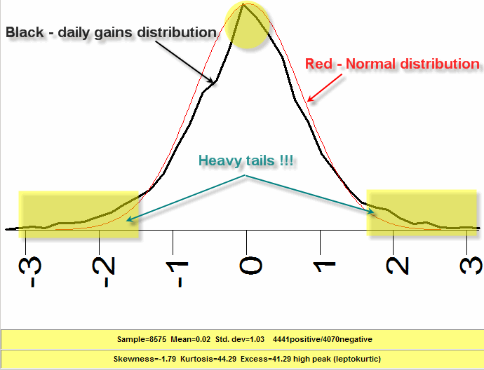
Now it is time to see the difference between ideal assumptions and a reality. We calculate a histogram for daily gains (Dow Jones 1975-2008 yy):

This histogram shows the probability of the next day movement; it is shown by the black curve. It differs from the normal distribution ("Gaussian bell") which is displayed by the red curve: the peak is sharper, and - a more important thing - there are too many points in the "tails" of this distribution. Mandelbrot called them "heavy tails".
For traders these "heavy tails" play the role of Pandora Box. They represent some price events that have not been taking into consideration yet; in other words, these zones represent risks. And this "not yet taken into account" territory is much more wider than we would expect usually (under normal distribution). Mandelbrot named this kind of distribution "wild randomness" in comparison to "mild randomness" we used to deal with. These "not yet taken into account" events can easily destroy all our constructions - like some mechanical trading system (that has been tested on 100 trades and provided 75 wining trades in the past) stops working for some unknown reason.
For a non-mathematician, this fact might look strange and not important: we
have two curves that look similar, the differences are minor. So why do they
lead to very different - and very dramatic - results, why is possible "The Formula
That Killed Wall Street"?
Let me show just one example. Make a bet with your friend: you pay him some
money if Dow Jones Industrial will drop more than 3% per day at least once
within 6 months. Why 6 months? It is simple; just conduct a statistical analysis
for Dow data from the year 1973 till 2007 (I excludes 2008-2009). Applying
normal statistical formulas and knowing that average daily change for Dow is 1%,
you find that this drop happens once in 3 years. Therefore, your risk is pretty
reasonable: 6 months against 3 years. After the bet starts, you will be
surprised to have more losses than expected. If you check your formulas,
everything is still Ok there. If you really look at all 3% drops that occurred
in 1973-2007 , there will be 31 of them, i.e. practically it happens every year.
Your risk is actually higher than anticipated. Why is such a difference between
statistical formulas and simple counting? The answer is in heavy tails
existence, in the fact that seldom events happen much more often.
I guess the same problem though with much more dramatic results presents in creating CDS (credit default swap) pricing model. What has happened there is very similar to my example. The possibilities of defaults have been definitely underestimated, and the result of it is known now to the whole World because the price of this misunderstanding is World's GDP.
I would like to finish this article citing the article I have started with:
The Gaussian cupola created the sort of financial
alchemy that made high-risk mortgages and credit card debt look like triple-A
rated gold.
March 27. 2009
Toronto, Canada