Verification of a projection line
Introduction
The usage of
astronomical/astrological phenomena gives us a totally different point of view regarding
trading and stock market modeling. The main player in this approach is a
PROJECTION LINE; this is the basis of astro trading. This is the cause of all
differences between �this approach and
any common tool of technical analysis. Technical analysis gives us a huge
variety of technical indicators � such as moving averages, RSI, stochastic
indicators, momentum indicators and many many other. All of them were
developed to help in revealing trading signals. With the projection line
we are focused on forecasting the sequence of whole market movements. This
feature gives to the trader an instrument that allows planning trader�s
activity on a different, deeper level.
In turn, a new problem
arises when we consider this approach. If we prefer technical analysis, we
would care to apply well adjusted technical analysis indicators to maximize our
profit. Dealing with the projection line, we have to know the way to
verify the workability of this projection line. How to do that? In this
article I have tried to share with you basic ideas regarding this issue. Due to
a lot of misunderstanding regarding this subject, I will try to follow the
explanation style used in the Universities at the time when I was a student. It
means that we start with the simplest definitions and move to more complicated
ones.
Definition: Projection
line
A projection line (curve)
is the prolongation of the price chart to the future, beyond the last available
at that moment price data. For example, today is July 5, 2011; the projection
line that we create should show the price projection after July 5, 2011. This
fact is the best way to distinguish between a projection line and some
technical analysis indicator. A projection line not only presents the price
chart in some special way (as technical analysis indicators do), it also models
a price chart and makes a prognosis of its future movement. How to do that is a
totally different story.
Definition: Forecast
horizon
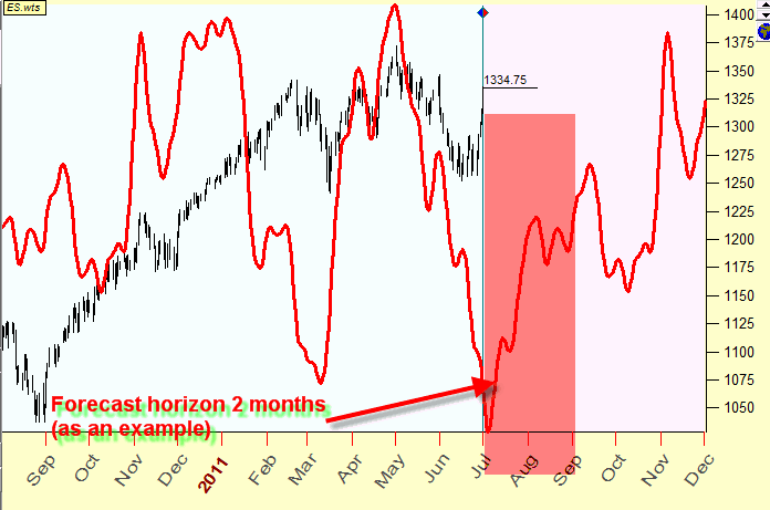
Usually the projection line
is able to forecast the price for some limited time period. As an example, the
forecast can be used for two month ahead, and after this period the projection
line should be recalculated. This is the reflection of the stock market reality:
the stock market constantly changes its structure, and accordingly the cycles
that can be found there may work differently at different moments of time. The
most stable cycles that I know are: the Annual cycle and 9-11years economics
Juglar cycle. Therefore, the forecast horizon is the period of time beyond the
last price data where we can trust our projection line:
Definition: Back
testing, In sample and Out of sample data, Learning Border cursor (LBC)
Back testing is a basis of
verification of the projection line. The idea of back testing is very simple:
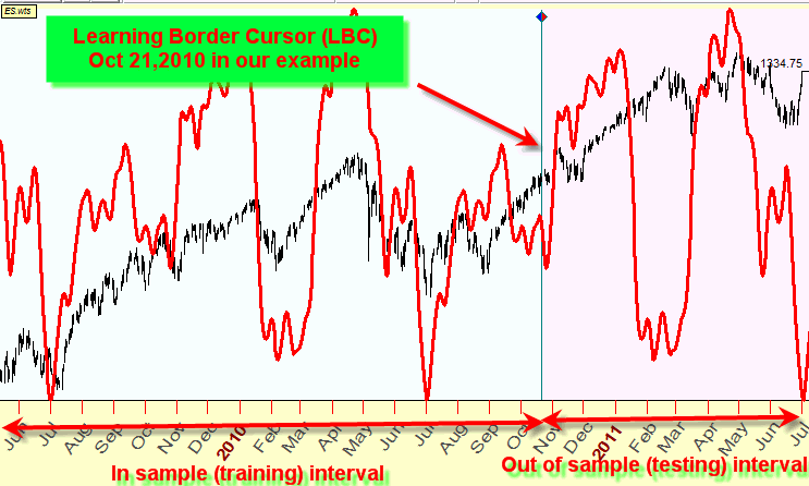
we take price history data set and break it on two parts � as it is done here:
The price history is divided
by two intervals: prior Oct 21, 2010 and after Oct 21, 2010. The
border between the two is called Learning Border Cursor or briefly LBC; the
name comes from Neural Network technology. In Neural Networks, they also call
the first (in sample) interval as Training or Learning interval, while the
second (out of sample) interval is also called Testing interval.
The idea of backtesting
procedure is quite obvious: we calculate a projection line using the data from
IN SAMPLE interval of the available price history (in our particular example it
would be price history data prior Oct 21, 2010). The OUT OF SAMPLE interval is
used to verify our projection line; i.e. we watch on the out of sample
portion of the price history (after Oct 21, 2010) how this projection line
would work in a real life when we do not know the future price movement.
And here we come across a
very important issue: we must be sure that there are no future leaks in this
procedure. Why is it so important? Just because it is so easy to get a perfect
forecast using some or the whole available price history from the out of sample
interval (in our example, the price history after: Oct 21, 2010). This is a
regular optimization procedure, nothing more; it indicates only that your tool
(a software, a system, a technique) really does what it should. (It should find
a model that fits perfectly to the data, no matter what data you use.) It is
the same thing as you have seen only a half of the movie and are guessing about
its end talking to a friend who saw it already several times; your friend has
no need to guess, your friend knows. So, the main issue here is the
honestly of developers of these systems. What can you do when somebody shows
you excellent pictures and promises high profits? Be on your guard. I can
recommend only that: do not believe any forecasts, strategies etc if they are
made post factum.
Let us go back to
backtesting.
In Timing Solution you can
set LBC at any place by making right mouse click anywhere on the Main Screen:
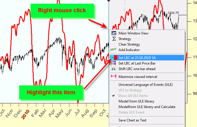
Do it several times,
setting LBC at different places. This way you can preview the workability of
your Turbo Cycles or Composite or any other model. The program does all
necessary (and believe me, very tiresome) calculations. All you need to do is
just set the LBC on different positions and watch the performance of your
projection line after LBC.
Definition: Walk Forward
analysis (WFA)
For some reason, though
backtesting idea is quite simple, I keep receiving similar questions regarding
it. One of the very frequently asked questions is: why should we move LBC many
times if we get a very good fitness on the testing interval for the very first
setting of LBC? My answer is: getting a perfect fitness between the price chart
and the projection line on out of sample (=testing) interval may be not enough.
We still may get the occasional coincidence between these two. To get more
reliable results, we have to set LBC on different dates and watch the
projection line after LBC.
Now, an interesting thought
came to my mind. Many people speak about back testing. And you will be surprise
how many different things they include into this idea. Here is a small list
what I was able to figure out:
1) Not any backtesting at
all (chart only) � when some system or technology is applied to the past data,
and excellent results in that kind of �back tests� are supposed to signify great
abilities of that system. Typical example is: today (July 5, 2011) somebody
says: "Look at my projection line; it works perfect since May 2011!" In
this situation, just ask him/her: "Why you have not shown your forecast in
May?" As I have mentioned above, post explanation tell nothing about
forecasting abilities of the system; it just shows how well that system can
reflect a well known reality (do you remember your friend who knows the movie�s
end because he/she saw it?).
2) Backtesting � looking
back at some forecast made in the past (documented!). For example, today (July
5, 2011) somebody shows his/her forecast from July 6 till the end of August
2011 (forecast for two months ahead). Put it (the forecast) into some place and
at the end of August 2011 compare it with the real price chart. Therefore, in
the end of August we will look back � at the forecast made in the beginning of
July. Even if the forecast is not good enough, there will be material to
discuss and learn.
3) Walk Forward analysis �
performing a backtesting procedure several times. For example, on January 1,
2011 we make a forecast till the end of January 2011, and in the end of
January we compare this forecast with the actual price. Then we perform the
same thing for February, March, ... December. Thus, in the end of December 2011
we will have the results of 12 independent backtesting procedures. Then we will
be able to analyze how often our forecast was right and how often it was wrong.
Definition: Sample Size
In the example above we
would conducted twelve backtesting procedures. It means that in our case the
sample size for our Walk Forward analysis is twelve. The more sample size is,
the more reliable results we get. There is only one restriction here: the
amount of available price history to conduct �good� backtestring.
Definition: Correlation
We use
correlation as a measure of coincidence between the projection line and the
price chart. Here is the definition made by Financial Forecast Center (http://www.neatideas.com/cc.htm).
What is
the Correlation Coefficient?
The
correlation coefficient concept from statistics is a measure of how well trends
in the predicted values follow trends in the actual values in the past. It is a
measure of how well the predicted values from a forecast model "fit"
with the real-life data.
The
correlation coefficient is a number between 0 and 1. If there is no
relationship between the predicted values and the actual values the correlation
coefficient is 0 or very low (the predicted values are no better than random
numbers). As the strength of the relationship between the predicted values and
actual values increases so does the correlation coefficient. A perfect fit
gives a coefficient of 1.0. Thus the higher the correlation coefficient the
better.
For
practical usage, you should know that:
1 � means an
ideal coincidence between two data sets (between your price chart and your
projection line);
0 - No
correlation. Two sets of data are not related.
-1 - anti-correlation;
it means that the predicted values "mirror" the actual values (or one
data set is the "mirror" for another one).
These are
examples:
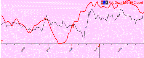
Positive
correlation (=0.5); these two curved lines show the same price movement (most
of the time). In other words, price goes up or down for both lines:
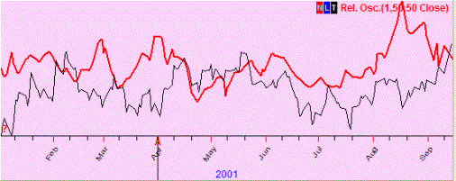
No
correlation (0.07); these two curved lines show totally different movements (if
one goes up, the other may go up or down and there is no regularity seen):
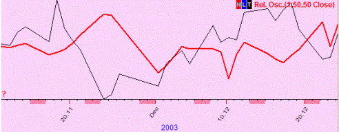
Negative
correlation (=-0.4); we observe the "mirror" effect (when one curved
line goes up, the other one goes down in most cases, and vice versa):
What correlation
is good enough? The more the better. Usually, the models that we analyze
provide 0.1-0.2 correlation. Sometimes it is more than that, but these results
are not stable. To be sure that this result is not accidental, it is necessary
to have a sufficient amount of price bars for calculating the correlation.
This
table shows the sufficient amount of price bars for different correlation
coefficients (Student's t-distribution):
|
Correlation |
Amount of price points to be sure that this result is not accidental |
|
0.1 |
390 |
|
0.2 |
100 |