written by Sergey Tarassov
General idea description for busy people
Playing with lag to find a leading indicator
Standard Intermarket templates
Customized Intermarket template
Appendix. General notes regarding Intermarket Analysis
This is a module with some history. It has been created 10 years ago, in 2009. Originally it was designed more as a research tool.
Then I have received lots of notes and wishes regarding this module. As a result, many new features have been incorporated there, and now a new version of this module is released.
What is Intermarket Analysis? The word "Intermarket" says it all: this type of analysis looks at several markets at the same time, as opposite to traditional analysis of financial markets where we look at one asset class or market individually. Comparing one market (which is our focus) to ther markets gives a better understanding of its strength and weakness and a valuable information regarding its possible direction. (Please see Appendix at the end of this article; it mentions brief ideas to explore and sources to study.)
One of the tools used in Intermarket Analysis is correlation. We would like to see the correlation 70% and more, positive or negative. However, the correlation is merely a constation of some fact. For trading, finding leading indicators has more practical value. It is an additional piece of information in making trading decisions. And this is what Timing Solution's Intermarket Analysis module does. It is available in Timing Solution Advanced version and in Pattern Recognition software. (Please keep in mind that access to Terra Incognita modules allows working with the most complete edition of Intermarket module. See details below.)
It is better to explain how this module works showing some practical example. Let us do it together.
For the analysis we have downloaded SNP500 since 1950. Our goal is to make a forecast for SNP500 using methods of intermarket analysis. So, to conduct intermarket analysis, the first step is downloading data for some other financial instrument or instruments. Then we look how these financial instruments (including SNP500) work together. To choose financial instruments for intermarket analysis, we may use any information (books, courses, etc.) Let us consider the idea that T-bonds are a leading indicator for stocks, and its effect is different at high and low interest rates. We can easily investigate this phenomenon with the new Intermarket module of Timing Solution software.
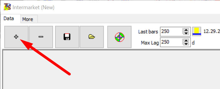
After downloading SNP500 index in the Main screen, run Intermarket module. It is in "Pattern" section. Click "+" button there to download a financial instrument that will be used for intermarket analysis:
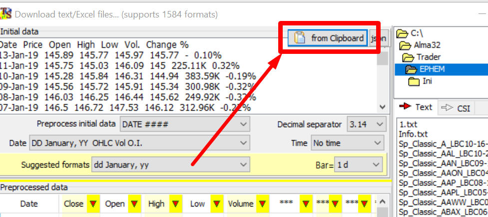
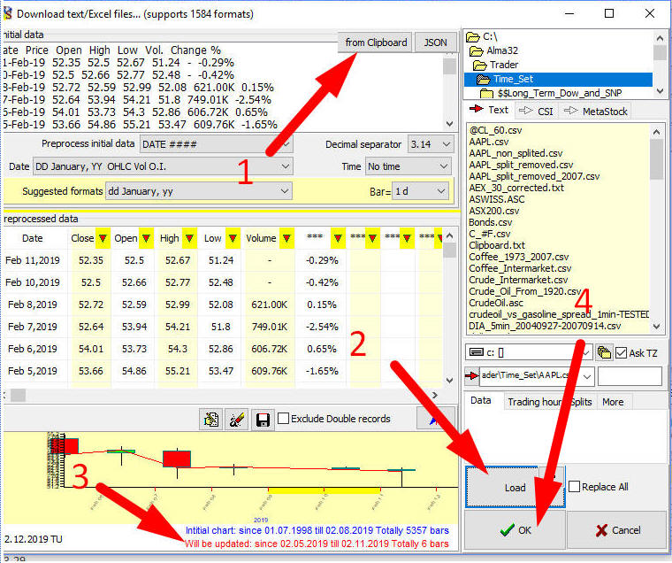
A standard for Timing Solution dialog box appears. It is designed for downloading price history from variety of sources: files, clipboard, Yahoo and Quandl services, eSignal, etc.
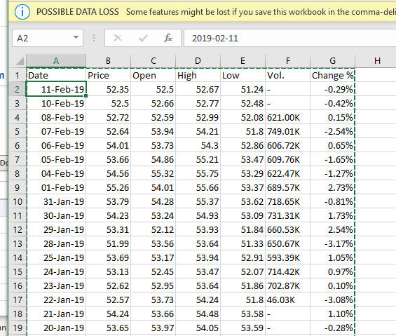
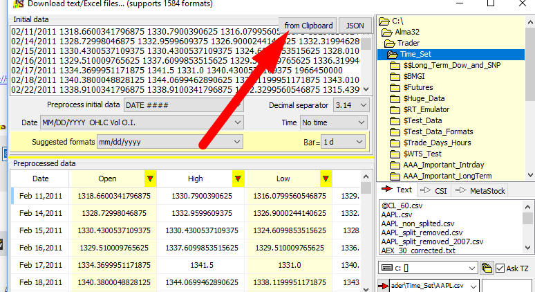
As an example, I use the data from free service https://www.investing.com . This service allows to load price history into Excel. We do that for 30 years US T-Bonds and copy the downloaded price history into the clipboard. When it is done, we download this price history data into Timing Solution by clicking "from Clipboard":
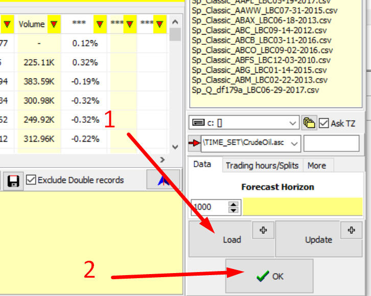
To confirm downloading, click "Load" and "OK" buttons:
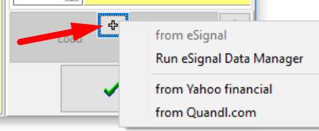
The same manner applies to downloading price history from some file or Internet using Yahoo/eSignal/Quand services. To do that, please use this button:
This is a standard procedure in Timing Solution; it is explained in this class: http://www.timingsolution.com/Doc/level_1/2.htm
Often data sources do not provide price history for more than a certain amount of years. It means that we should download price history from different sources covering different time intervals. In this case instead of using "Load" button click "Update" button: new pieces of price data will be added to already downloaded price history.
When it is done (data are downloaded for both, SNP500 and T-bonds, as an example), in the Intermarket module window we can see a panel for T-Bonds. The controls there allow to conduct intermarket analysis for T-Bonds versus SNP500:
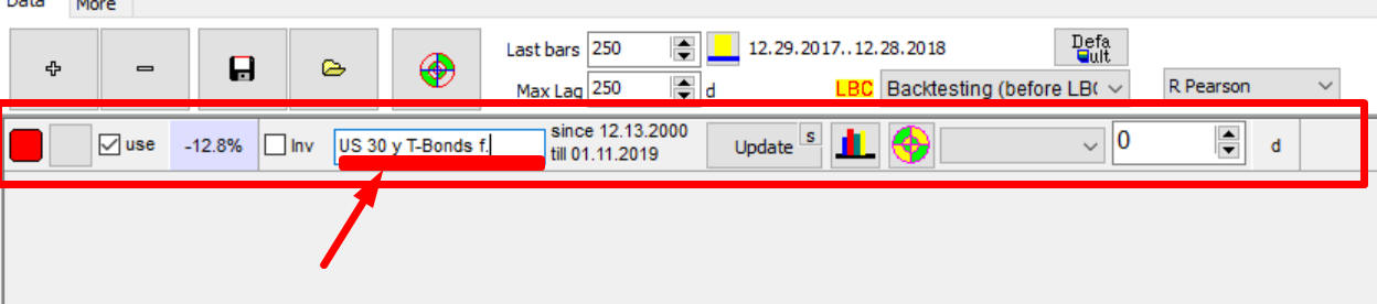
It is recommended to type there the name of a downloaded financial instrument, it serves as a reminder.
Look at the Main screen now:
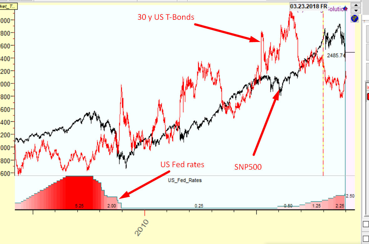
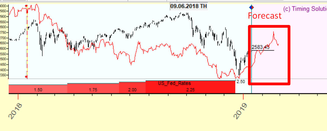
There is a chart there for downloaded SNP500 index, a red curve that represents US T bonds and a red diagram in the bottom panel that shows US Fed rates history.
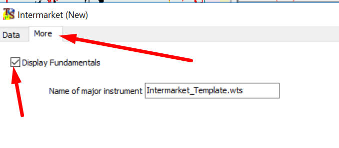
To disable US Fed rates information, set OFF "Display Fundamentals" in "More" tab:
Is there any correlation between these financial instruments? Usually researchers display both charts (SNP and T bonds in our example) and watch how they move together. Charts are considered correlated - if they show approximately the same movement, i.e. if one instrument goes up, another instrument shows up movement as well and vise versa. They are anti correlated - if they show opposite movement, i.e. if one goes up while another goes down and vise versa. Such visual analysis can be done by zooming the price chart and watching a mutual behavior of these two charts (SNP500 and T-Bonds in the example). However, to see the whole picture we should conduct a more formal analysis.
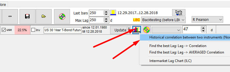
To research a correlation between SNP500 and T-Bonds, click this button and in the pop-up menu choose "Historical correlation" item:
In a moment the correlation chart appears:
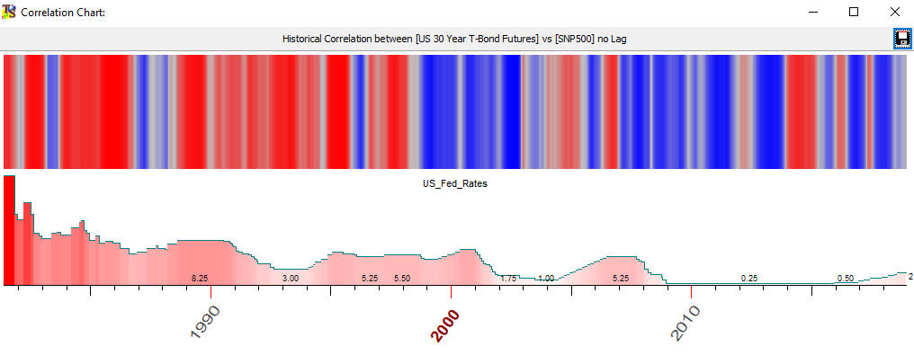
The red periods there show dates when SNP500 and T-Bonds are correlated in a positive way, i.e. when they move in the same direction. Blue zones show anti correlated periods i.e. dates when these financial instruments move in opposite direction.
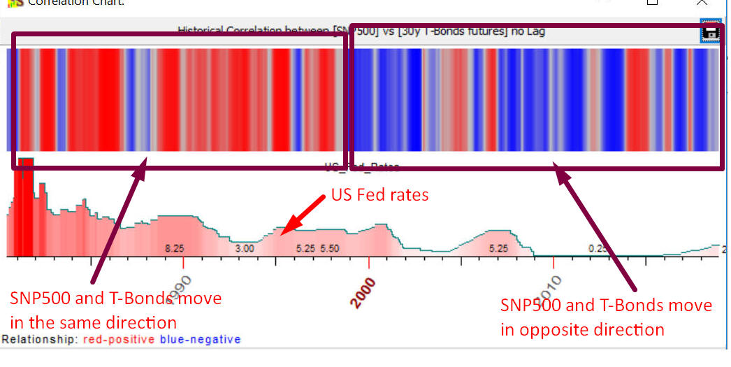
In this example SNP500 and T-Bonds correlated positively till 1999; this is a period of high FED rates mostly. Since 1999 we have the opposite picture: SNP500 and T-Bonds correlate in a negative way, and rates were mostly low.
The brighter zones there correspond to higher correlation/anti correlation. Moving a mouse cursor through the correlation chart, we can see the degree of this correlation/anti correlation for different dates:
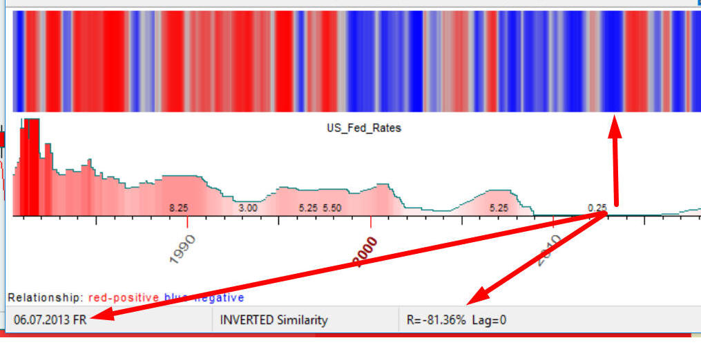
The diagram below shows that in the middle of 2013 SNP500 and T-Bonds mostly moved in opposite way (inverted similarity), and the correlation is high negative -81%.
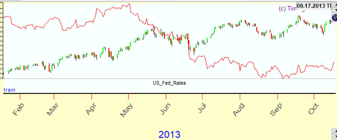
This is the price chart for this period:
The correlation between markets gives a valuable information. However, there are more interesting things in the Intermarket Analysis.
The main goal of intermarket analysis suggested by Timing Solution is finding a leading indicator - the indicator that moves ahead, providing some useful tips regarding possible future movements. In the example above, we have already tried to find a correlation between two different markets (charts, financial instruments). When a direct comparison does not work, we may try working with shifted charts. This approach has a significant advantage: if we find a lag, it means that we have some time to be prepared for the next market move.
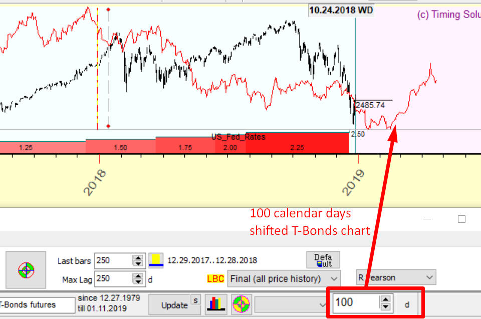
Look at this example. There we have shifted forward T-Bonds chart on 100 calendar days, the lag = 100 days:
We may change lag values to find a better correlation between the researched financial instrument (SNP500 in our case) and the shifted chart (T-Bonds) . What lag is better for forecasting -10, 50, ..20 days - or some other lag? Let me say from the very beginning: there are no rules here that work forever (that is always in finance, no surprise here). However, applying different mathematical approaches, it is possible to get the best lag, and below you will find the description of these techniques.
Before going further, some definitions must be considered.
The research of the relations between a financial instrument that we consider as a leading indicator (2) to the financial instrument whose behavior we would like to forecast (1) is called as "2 versus 1". These numbers, 1 and 2, relate in the program to the download routine. In our example, 1 relates to SNP500 and 2 relates to T-Bonds. We consider T-Bonds being a leading indicator to SNP500. So, we would research "T-Bonds versus SNP500".
Analyzed interval (order) - pay attention to this parameter. It is the time interval where the program calculates a correlation for assumed leading indicator versus the financial instrument whose behavior we would like to forecast. In our example, it is the interval where the program calculates a correlation for T-Bonds versus SNP500. By default it is set to 250 bars:
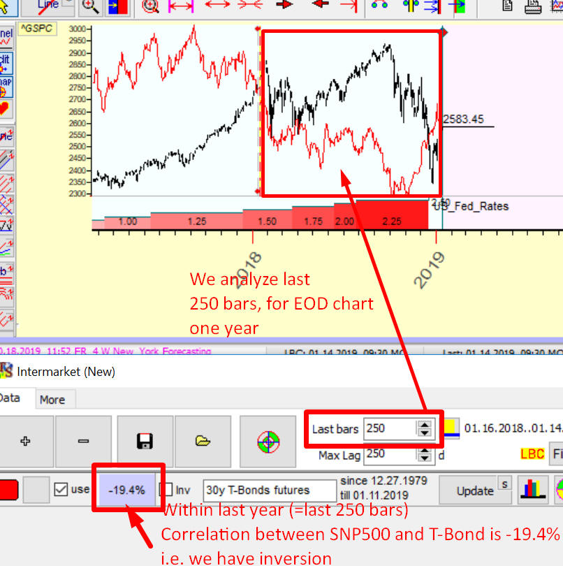
The program calculates a fitness between these two financial instruments within the last year (as the last 250 bars of EOD chart make about 1 calendar year):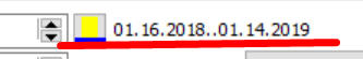
We have the negative correlation here = -19.4%, so these instruments are more inverted.
Now shift T-Bonds price chart one calendar day ahead and watch how the fitness between SNP500 (last 250 bars) and the shifted T-Bonds chart has changed.
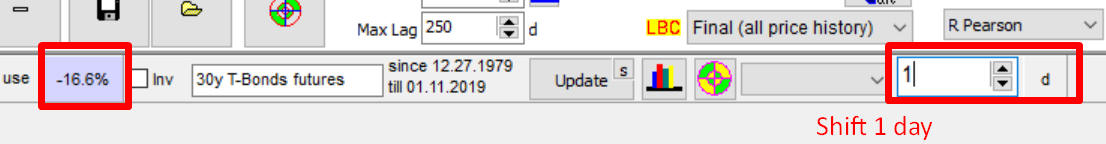
The correlation now is -16.6%. Then let us do 2 days shift. The correlation=-15.1%. And so on...
To get a full picture of how the correlation for shifted T-Bonds versus SNP500 changes with a change of a lag, do this:
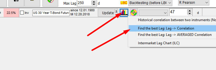
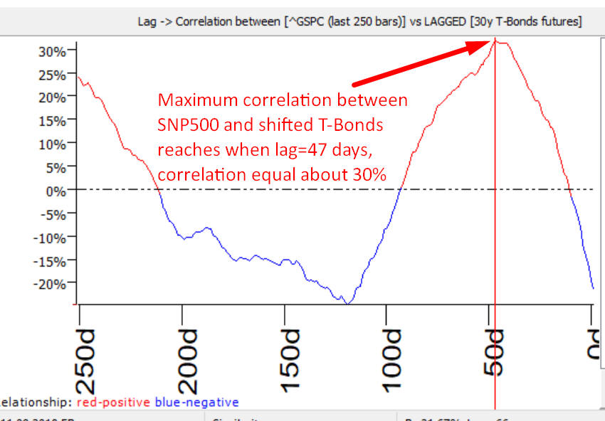
The diagram appears that shows how the correlation for shifted T-Bonds versus SNP500 varies while we change the lag:
 shifted
The diagram above shows that at lag=47 days the correlation reaches its maximum value about 30%.
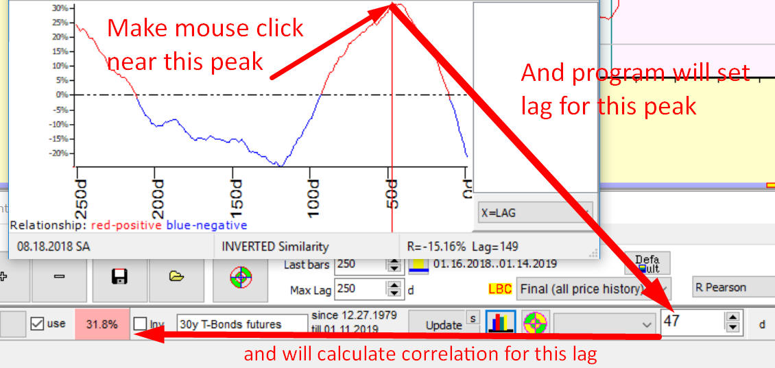
To simplify this procedure, make a mouse click around the peak on this diagram. The program automatically will set the lag for this peak (47 days) and will calculate the correlation (31.8%):
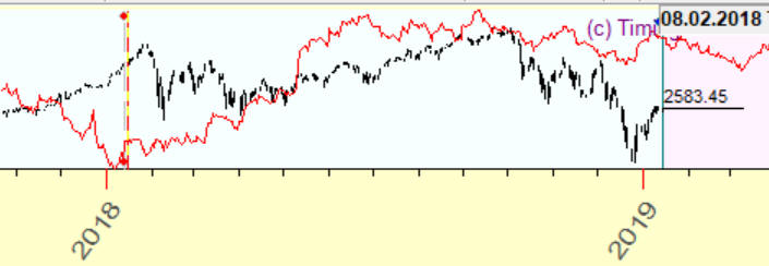
Accordingly in the Main screen this 47 calendar days shifted T-Bonds chart will be shown, and this information may be used as a forecast for SNP500:
You can also use "Optimize" button
It will calculate the best lags to choose any of them:
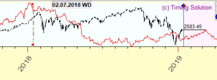
Reminder - when you use a lag with a negative correlation it means that SNP500 and shifted T-Bonds charts are inverted. In this case it would be better to invert the intermarket chart:
Or at least you should remember about the inversion.
One more feature to play with lag. You can vary the lag by dragging the price chart with the mouse. In order to do that, click this button:
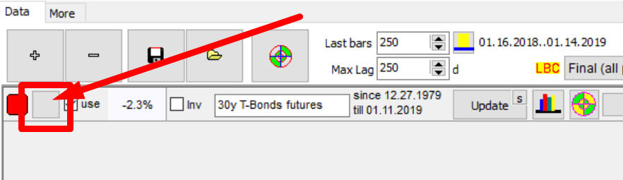
When you click this button the very first time, the eye image will appear on the button, as well as time and price scale for T-Bonds.
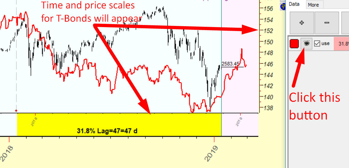
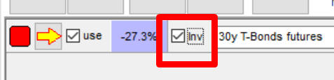
Click this button once again, and yellow arrow image will appear on it:
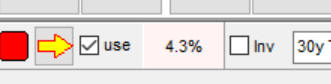
Now you can shift the T-Bonds chart by dragging the mouse cursor. While you drag this chart, the lag value and the correlation vary as well.
This button works in three modes: no image - the standard mode,  eye image - displays time and price scale for the compared instrument and
  arrow image - allows to drag its chart manually.
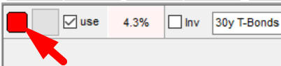
Color/thickness: click on this button to change the color or thickness of the chart:
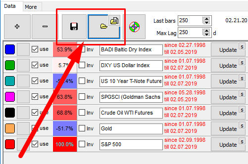
Use: The program is able to conduct intermarket analysis comparing many financial instruments at once. You can create as many intermarket charts as you want. Sometimes not all of them are needed. In this case it is useful to hide some charts from the screen. This can be done with "use" option:
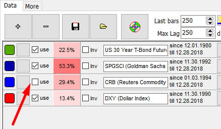
In this example we have already downloaded T-Bonds, two commodity indexes and Dollar index. And later, for some reason, we decide to remove one commodity index. In order to do that, mark that index as not USED (uncheck it):
After that click "-' button and in the pop-up menu choose the first option:
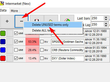
The second option serves in case you want to delete all items and start new Intermarket Analysis from scratch.
Inverted chart: to invert the price chart, use this option:
Here are examples of two charts:
Normal view
Inverted
To run ILC, do this:

This module takes some time for calculation. It analyses all available price history trying to reveal leading and lagging indicators for any pair of financial instruments.
This is how ILC chart for T Bonds looks:
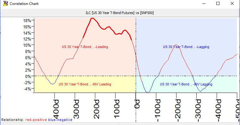
You need to watch here the highest peak. In the example it is in the left upper side. The left side means that T-Bonds is leading indicator for SNP500. The upper part/zone means that this is normal, not inverted indicator.
The peak here corresponds to the lag=210 calendar days. Clicking a mouse button around this peak sets this lag value in the program:
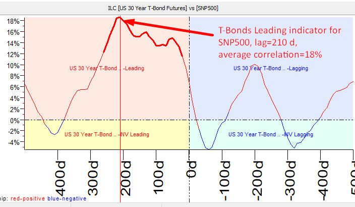
In the Main screen the corresponding shifted forward on 210 days T-Bonds chart will appear. Because T-Bonds is a leading indicator, it can be used for forecasting future SNP500 moves. The forecast power of this leading indicator is 18%, not bad. This is an averaged correlation between analyzed and lagged charts.
Here is an example of the inverted leading indicator; this is ILC for Dollar Index versus SNP500:
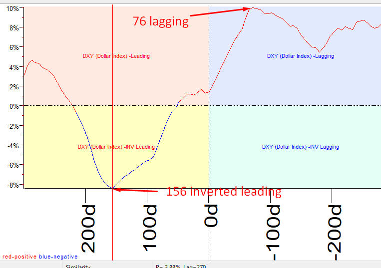
Dollar index is the inverted leading indicator for SNP500 with the lag of 156 calendar days. The same indicator can be considered as lagging with the lag=76 days.
This information can be read this way: a lowering dollar index drives the stock market with the lag of 156 days (leading anti-correlation). And when the stock market is getting higher, the dollar index is getting higher as well with the lag of 72 days (a lagging correlation). The same indicator here plays a role of leading and lagging indicator, it shows the phases of some business cycle. However, the forecast power for this indicator is not high: accordingly 8 and 10%, i.e. the averaged correlation for this index is -8% (minus because it is inverted) and 10%.
You can conduct more advanced research. Try another example: calculating ILC for the period of super low interest rates (2009-2016). When you run ILC chart, the program shows this box where you may specify parameters for ILC chart:
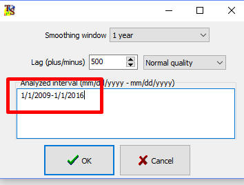
You can specify the analyzed interval there (if this box is empty, program analyses all available price history). This is how ILC T-Bond vs SNP500 for super low rates period looks:
The new strong peak with Lag=0 appeared. It means that when FED rates are low, we have a strong anti-correlation between T-Bonds and SNP500. If we calculate ILC for the period of high rates, we get the opposite picture: a strong positive peak around zero lag, i.e. the strong correlation between T-Bonds and SNP500. Pay attention, at the same time 210 days shifted chart can be used as a leading indicator for SNP500.
After the price history was downloaded, there is no need to download it every time when working with the same financial instrument. Instead, the price history information can be updated. The features designed for it are described below.
Updating: to update the existing price history, click "Update" button:
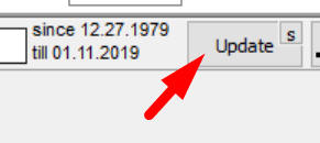
Pay attention to a panel "since...till"; there you can see always the downloaded interval.
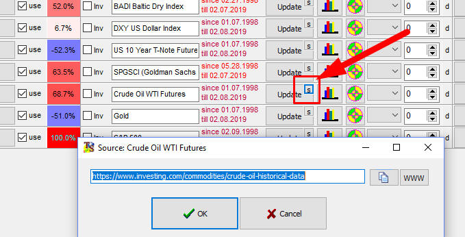
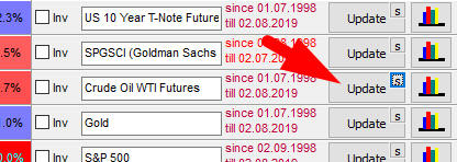
Source: clicking this small "S" button, you may store some custom information regarding the source of downloaded price history data.for this financial instrument:
For your convenience, we have added a possibility for Internet sources to open the corresponding website right from this window, by clicking "WWW" button:
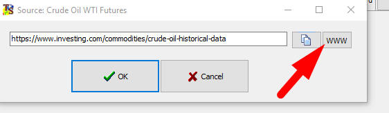
As an example, the crude oil price history has been downloaded from the website www.investing.com. To update the price history, click "WWW" button. You get the page with the latest price history provided by that source:
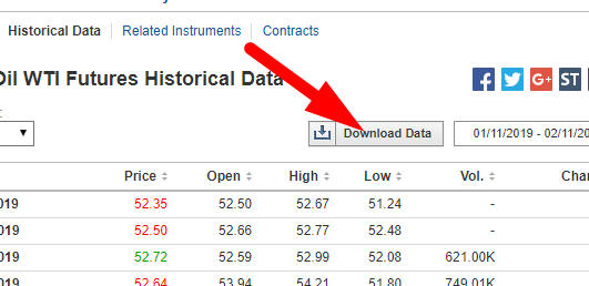
Then click "Download Data" button there to get Excel file with the data:
To move this information from Excel to Timing Solution, it should be put into the clipboard. We do that by clicking Ctrl-A to select all data in this Excel table and then clicking Ctrl-C to put this data into the clipboard (another way is to do the right mouse click over selected data and then choose "Copy" in the popup menu). Now the latest price history from the website www.investing.com is in the clipboard; we are ready to update the existing price history in the Intermarket module.
Click "Update" button:
Click "from Clipboard" button to paste this data (1); then click "Load" button to download this piece of price history from clipboard into Timing Solution (2). Look at the bottom of this window, to ensure that downloaded data is Ok (3) and click "Ok" button to confirm this procedure (4). These 4 steps are shown here::
Sometimes when you click "WWW" button, you may get this message:
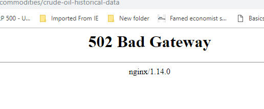
It means that you probably need to log to the original website. In this case, simply run your data source website (as an example, https://www.investing.com/) and enter there your login information. After that you can click "WWW" as many times as you need within one session.
Your data source might be Yahoo financial service; in this case you get something like this:
Clicking "WWW" button, you get this information, the price history, in JSON format:
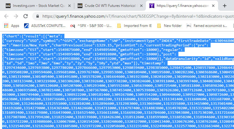
Simply put all this information into the clipboard as it is explained in the previous example and then paste it into Timing Solution (and click "Load" and after that click "Ok"):
The program automatically recognizes Yahoo JSON format.
Here is the video with a brief explanation how to update the price history for Intermarket module:
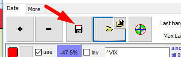
As so far, we have discussed the basics of Intermarket Analysis and how it works in Timing Solution software. We know that we need to create a chart of the financial instrument that we plan to trade and charts of other financial instruments that may serve as leading or lagging indicators. We are able to deal with correlation and know how ILC (Intermarket Lag Chart) works. And the day is over. We closed our computers - just to come back tomorrow and start that again. To save your time and make your life easier, we suggest to work with templates. There is no need to download same charts again and again, no need to remember all parameters that you used for your Intermarket models. In a real life, you would like to work instead with some pre-defined set of intermarket financial instruments comparing some or all of them against the financial instruments you plan to trade. You can save your intermarket model as a template and later open it and apply for any financial instrument you trade. In order to do that use these buttons:
The good thing with templates is that you can once define what financial instruments you may need to consider, download them once and later update only those that you really need to work with. Timing Solution has provided two options for that: using a standard template (updated once a week by Timing Solution Support team) and creating your own customized template.
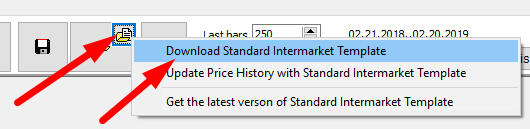
The program downloads this template from Internet. When you do this procedure the very first time, your security system will ask to allow Timing Solution to get access to Internet (obviously, click yes).
When the latest version of the standard Intermarket template is downloaded, click this option to release its content to Timing Solution:
You will get the list of financial instruments ready for your Intermarket analysis:
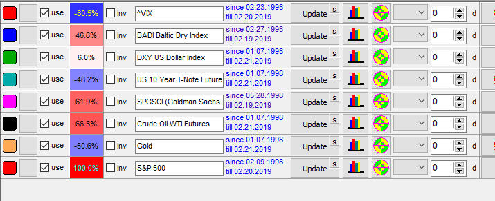
This list is based on our knowledge and the experience of Timing Solution users. However, you may not need some instruments here. As an example, if you would like to forecast Gold and find leading indicators for it, you do not need Gold in the Intermarket module. So it should be deleted as useless (how to do that is explained above).
You can create your own Intermarket template. It may include any financial instrument that you would like to test and as many of them as you want. The procedure is simple:
1) Download any financial instrument that you plan to use often in Intermarket module;
2) Update its price history in a regular way;
3) Save your Intermarket template:
A. Updating through the standard Intermarket template
The price history in the standard Intermarket template is updated once a week by our TS Support team, and accordingly you can also update the price history in your TS worksheets (if these include Intermarket models with the elements of the standard Intermarket template). In order to do that:
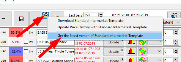
1) Download the latest standard Intermarket template:
2) Do this:
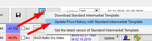
Only price hiistory will be updated; all your parameters like lags stay the same. We recommend to do this procedure once a week if you work with Intermarket module; you will get the latest available price history. It saves your time.
B. Updating thorugh a customized Intermarket template
You can also update the price history manually, for each financial instrument, one by one, using the process explained above.
It is time consuming, though. To simplify this task, you can use your Intermarket template.
Do that this way:
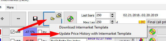
This procedure works exactly the same as updating price history through the standard Intermarket template
January 10 - February 21, 2019
Toronto, Canada
Leading Indicators
| Interamarket Lag Matrix | ||||||||||||||||||||||||||||||||||||
| LEADING indicators, for example for Dow Jones leading indicators are (red colored cells): Gold lag=134 days, Inverted Cocoa Lag=51 days, Inverted CHFEUR Lag=73 days | ||||||||||||||||||||||||||||||||||||
| Dow Jones | Gold | Silver | Platinum | Copper | Wheat | Rough Rice | Soybean Meal | Soybean Oil | Feeder Cattle | Live Cattle | Cocoa | Coffee | Cotton | Lumber | Sugar | Crude Oil | Heating Oil | Natural Gas | USA T Bonds | 10y T-Note | 5y T-Note | 2y T-Note | EURUSD | JPYUSD | EURJPY | GBPUSD | GBPEUR | CHFUSD | CHFEUR | CADUSD | CADEUR | AUDUSD | AUDEUR | NZDUSD | NZDEUR | |
| Dow Jones | -134 | INV -51 | INV -73 | |||||||||||||||||||||||||||||||||
| Gold | INV -120 | INV -126 | INV -87 | INV -89 | -114 | |||||||||||||||||||||||||||||||
| Silver | -50 | -47 | INV -111 | INV -90 | INV -14 | INV -136 | ||||||||||||||||||||||||||||||
| Platinum | -50 | -44 | -47 | INV -146 | -40 | INV -91 | ||||||||||||||||||||||||||||||
| Copper | -137 | -72 | INV -117 | |||||||||||||||||||||||||||||||||
| Wheat | -50 | INV -82 | INV -82 | INV -64 | INV -70 | |||||||||||||||||||||||||||||||
| Rough Rice | -56 | -28 | -16 | -80 | -33 | INV -25 | -47 | |||||||||||||||||||||||||||||
| Soybean Meal | INV -109 | |||||||||||||||||||||||||||||||||||
| Soybean Oil | -57 | INV -74 | ||||||||||||||||||||||||||||||||||
| Feeder Cattle | -147 | |||||||||||||||||||||||||||||||||||
| Live Cattle | -140 | INV -95 | -99 | -88 | ||||||||||||||||||||||||||||||||
| Cocoa | -97 | -40 | -40 | -52 | -42 | -69 | INV -139 | -47 | -38 | |||||||||||||||||||||||||||
| Coffee | -113 | -138 | ||||||||||||||||||||||||||||||||||
| Cotton | -49 | -48 | -48 | -31 | -36 | |||||||||||||||||||||||||||||||
| Lumber | INV -12 | -145 | -16 | |||||||||||||||||||||||||||||||||
| Sugar | INV -120 | INV -111 | -66 | -82 | ||||||||||||||||||||||||||||||||
| Crude Oil | -108 | -79 | -86 | -22 | INV -131 | |||||||||||||||||||||||||||||||
| Heating Oil | -121 | -66 | -30 | -38 | INV -138 | INV -131 | INV -132 | |||||||||||||||||||||||||||||
| Natural Gas | -86 | -86 | -94 | INV -29 | INV -42 | -61 | -56 | -56 | -85 | -91 | INV -84 | -88 | -58 | -97 | -112 | |||||||||||||||||||||
| USA T Bonds | INV -14 | INV -36 | -132 | -126 | INV -47 | |||||||||||||||||||||||||||||||
| 10y T-Note | INV -18 | INV -43 | INV -87 | -110 | -131 | INV -48 | ||||||||||||||||||||||||||||||
| 5y T-Note | INV -18 | INV -43 | INV -12 | INV -86 | -130 | |||||||||||||||||||||||||||||||
| 2y T-Note | INV -50 | -125 | INV -12 | INV -86 | -130 | |||||||||||||||||||||||||||||||
| EURUSD | ||||||||||||||||||||||||||||||||||||
| JPYUSD | INV -49 | INV -13 | INV -64 | |||||||||||||||||||||||||||||||||
| EURJPY | -116 | -111 | INV -37 | |||||||||||||||||||||||||||||||||
| GBPUSD | INV -132 | INV -134 | ||||||||||||||||||||||||||||||||||
| GBPEUR | -118 | -10 | ||||||||||||||||||||||||||||||||||
| CHFUSD | INV -108 | INV -128 | ||||||||||||||||||||||||||||||||||
| CHFEUR | -145 | INV -22 | INV -34 | INV -42 | ||||||||||||||||||||||||||||||||
| CADUSD | -13 | -33 | ||||||||||||||||||||||||||||||||||
| CADEUR | -132 | -122 | -125 | -13 | -136 | INV -55 | -140 | |||||||||||||||||||||||||||||
| AUDUSD | INV -82 | |||||||||||||||||||||||||||||||||||
| AUDEUR | -111 | -132 | INV -52 | -132 | ||||||||||||||||||||||||||||||||
| NZDUSD | INV -84 | |||||||||||||||||||||||||||||||||||
| NZDEUR | -142 | |||||||||||||||||||||||||||||||||||
According to Investopedia, Intermarket Analysis is looking not at one asset class or financial market individually, it looks at several "to determine the strength or weakness of" the financial market or asset class that we analyse. It gives you a general sense and direction. There are different approaches to intermarket analysis, including mechanical and rule-based. A simple correlation study is the easiest type of intermarket analysis to perform. Any reading sustained over the +0.7 or under the –0.7 level (which would equate to 70 percent correlation) is statistically significant. Also, if a correlation moves from positive to negative, the relationship would most likely be unstable, and probably useless for trading. The most widely accepted correlation is the inverse correlation between stock prices and interest rates, which postulates that as interest rates go up, stock prices go lower, and conversely, as interest rates go down, stock prices go up.(https://www.investopedia.com/terms/i/intermarketanalysis.asp)
Wikipedia says: In finance,intermarket analysis refers to the study of how "different sectors of the market move in relationships with other sectors." Technical analyst John J. Murphy pioneered this field.
Some basic ideas from studying J.Murphy, Intermarket Analysis:
1) All markets are linked, domestically and globally;
2) No market moves in isolation;
3) Analysis of one market should include all the others;
4) The four market groups are stocks, bonds, commodities, and currencies (TS: it means that we have a lot of different financial instruments to work with)
5) Observations made by Mr. Murphy and confirmed by other authors:
5.1) The dollar and commodities trend in opposite directions;
5.2) Bond prices and commodities trend in opposite directions;
5.3) Bonds and stocks normally trend in the same direction;
5.4)Bonds peak and trough ahead of stocks;
5.5)During deflation, bond prices rise while stocks fall;
5.6)A rising dollar is good for U.S. bonds and stocks;
5.7)A weak dollar favors large multinational stocks;
5.8)A rising commodity/bond ratio favors inflation-type stocks including gold, energy, and basic material stocks like aluminum, copper, paper and forest products;
5.9)A falling commodity/bond ratio favors interest rate-sensitive stocks including consumer staples, drugs, financials and utilities.
Two last items are related to another approach to Intermarket Analysis, Sector Rotation. It reflects the observation and comparison of different markets in regards to the of Business Cycle. Intermarket module of Timing Solution does not include Sector Rotation. Our approach is reflected in another software, TS Scanner.
Here is the explanation of Business Cycle according to Intermarket Review by Martin J. Pring. The business cycle is shown as a sine wave. The first three stages are parts of an economic contraction (weakening, bottoming, and strengthening). At the beginning of Stage 3 the economy is in a contraction phase, but strengthening after a bottom. As the sine wave crosses the centerline, the economy moves from contraction to the three phases of economic expansion (strengthening, topping, and weakening). Stage 6 shows the economy in an expansion phase, but weakening after a top. These are some Business Cycle Rules for inflationary environment:
At Stage 1 (contracting economy) bonds turning up as interest rates decline. (Explanation: Economic weakness favors loose monetary policy and the lowering of interest rates, which is bullish for bonds.)
Stage 2 marks a bottom in the economy and the stock market. (Explanation: Even though economic conditions have stopped deteriorating, the economy is still not at an expansion stage or actually growing. However, stocks anticipate an expansion phase by bottoming before the contraction period ends.)
At Stage 3 Stocks are rising and commodities turning up. (Explanation: A vast improvement in economic conditions as the business cycle prepares to move into an expansion phase.)
Stage 4 marks a period of full expansion. Both stocks and commodities are rising, but bonds turn lower. (Explanation: The expansion increases inflationary pressures. Interest rates start moving higher to combat inflationary pressures.)
Stage 5 marks a peak in economic growth and the stock market. Stocks peak first followed by commodities' peaks. (Explanation: Even though the expansion continues, the economy grows at a slower pace because rising interest rates and rising commodity prices take their toll. Stocks anticipate a contraction phase by peaking before the expansion actually ends. Commodities remain strong and peak after stocks.)
At Stage 6 stocks and commodities move lower. (Explanation: This is a deterioration in the economy as the business cycle prepares to move from an expansion phase to a contraction phase. Stocks have already been moving lower and commodities now turn lower in anticipation of decreased demand from the deteriorating economy.) Keep in mind that in an inflationary environment stocks and bonds advance together in stages 2 and 3. Similarly, both decline in stages 5 and 6. This would not be the case in a deflationary environment, when bonds and stocks would move in opposite directions.
Besides books by J.Murphy and M.Pring, you may want to look at works by Louis B. Mendelsohn, Markos Katsanos, and Ashraf Laïdi.
However, they mostly observe market pairs and make conclusions on practical examples at different times. Many of their ideas can be tested with Timing Solution new Intermarket module.