Digital Signal Processing (DSP) in Timing Solution
Introduction
DSP module allows to reveal cyclic phenomena in financial data. In Timing Solution, our basic software, there are many modules devoted to cyclic analysis. Is DSP module something new or the same things can be done with existing modules? To answer this question, I begin the explanation discussing the difference between DSP and existing spectral analysis modules. To be precise, we will speak here not about DSP science in general, but about only one of its features that allows to reveal a dominant cycle (Hilbert Transform). This approach is called here as DSP.
DSP sees the price movement as a spinning wheel; this wheel rotates with different speed at different moments of time, and it is important to remember that this is ONE and the same wheel. We put all cyclic phenomena into one wheel, and this wheel is called a dominant cycle.
Spectral analysis allows to reveal dominant cycles, too. But it works totally different: it sees the price movement as a superposition of several wheels, and each wheel there rotates with its own speed. We can compare DSP models with some musician virtuoso who is able to play a symphony on the piano only, simulating different instruments. While the spectrum module is the orchestra where everybody plays his or her part.
This difference causes some disadvantage of DSP approach: if our "musician" has to imitate too many instruments. there is a risk to play some parts incorrectly or to miss something; noise is very strong in this model. However, this approach has its advantages as well: it allows to create technical analysis indicators based on the dominant cycle. These new smart indicators were developed by John Ehlers. In other words, DSP approach is very good for creating smart indicators of Technical Analysis, while spectral analysis approach is better to use to create a projection line (i.e., to model the market behavior). (You can read about spectral analysis approach here: http://www.timingsolution.com/TS/Study/Classes/class_spectr_1.htm; look also Turbo Cycles module http://www.timingsolution.com/TS/Study/Turbo_Cycles/).
Techniques description
Now, let's discuss DSP module. It is in Terra Incognita project conducted by Timing Solution team.
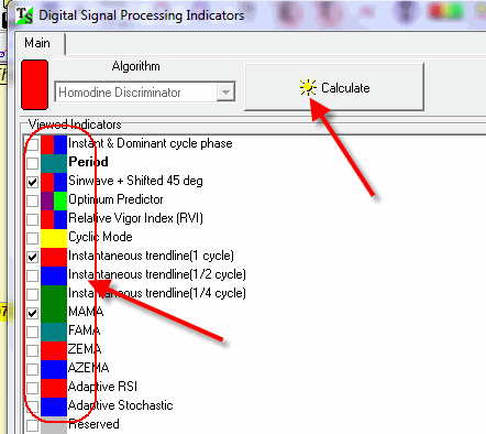
To run this module, follow this path: "TI"=>"Digital Signal Processing Indicators" menu:

Click "Calculate" button and then check mark those indicators that you want to be displayed in the Main screen.
DSP module has several important components.
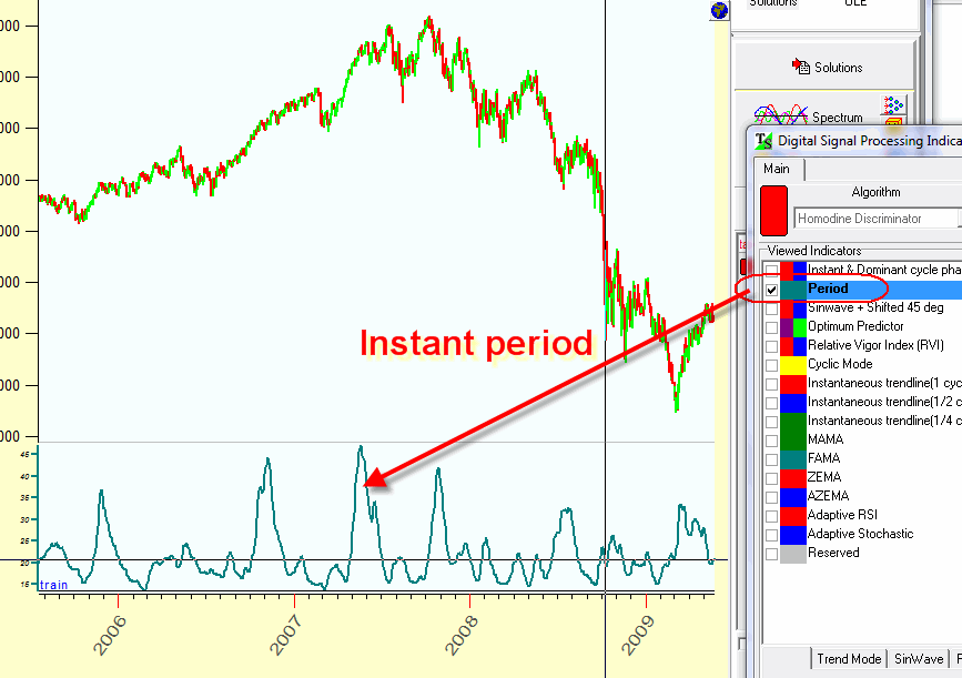
Instant Period: The central feature of DSP is the possibility to reveal an instantaneous dominant cycle, i.e. to find its period. You can see how the period of a dominant cycle changes in time:
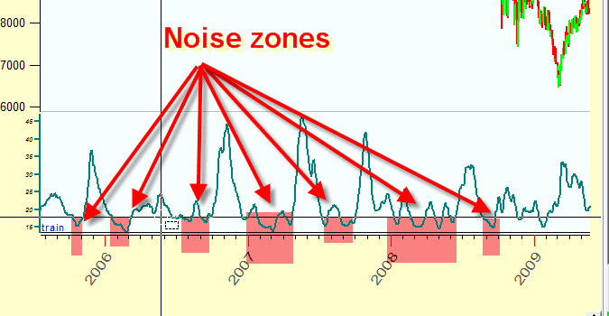
Short term cycles (i.e. cycles with the small period) contain more noise, so these zones are more risky. The zones where long term cycles are in play are more predictable:
The lag of this indicator is 7 bars.
Sin wave indicator. Having instantaneous period, we can create a sin wave indicator based on this cycle. You can take this sin wave indicator as a trajectory of the rotating wheel which represents the price movement. Here you should pay attention to the moments of the intersection of a red and a blue sin waves, these points often indicate CIT moments:
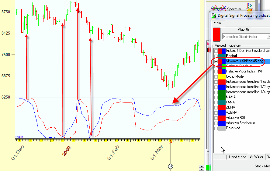
The best thing about this indicator is that it has no lag
Also pay attention to the fact that the sin wave indicator allows to specify trend and cyclic zones:
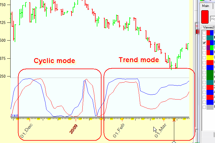
If stock market is in trend mode, the phase changes very slowly, so the sin wave changes slowly as well.
Optimum Predictor: The possibility to calculate the period of the dominant cycle leads to another step: we can create one more indicator that is able to predict upcoming turning points. This is Optimum Predictor indicator. This is how it looks:
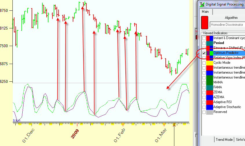
As Ehlers states the most amount of buy and sell signals occurs when these two lines cross, though it would be better to use this indicator together with other rules to eliminate false signals.
Relative Vigor Index. It works in the same manner as the previous one, but it is more sharp:
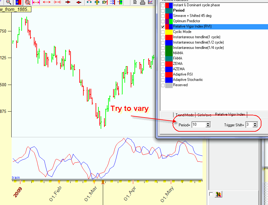
I recommend to vary the period of RVI index and the shift for the trigger line.
The knowledge of a period of the dominant cycle allows to calculate the moving average based on this cycle. The advantage of this approach is that the moving average based on this instant dominant cycle allows to remove a cyclic component in a smart way, after that this moving average can be used as a basis of the moving crossover system.
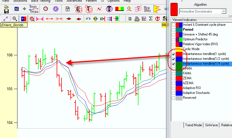
Instantaneous trend line - this is a simple moving average with the smoothing window equal to the period of the dominant cycle.
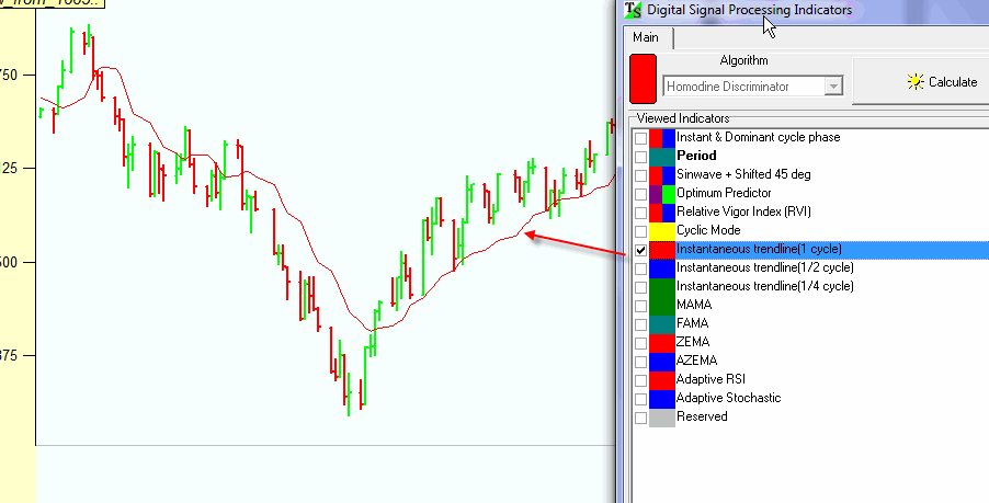
The lag of this MA is a half of the dominant cycle.
J. F. Ehlers recommends to use the crossover of two moving averages: the instantaneous trend line based on the entire cycle and the instantaneous trend line based on a quarter of the dominant cycle. The half period trend line may be used as a confirmation signal:
MAMA and FAMA (Mesa adaptive moving average and Following adaptive moving average) allows to calculate a moving average using more advanced algorithms. It is based on exponential moving averages, the smoothing coefficient here changes according to the speed of the rotation of our wheel (i.e rate of change of the phase).
You can consider MAMA as a slow moving average while FAMA is a fast moving average:
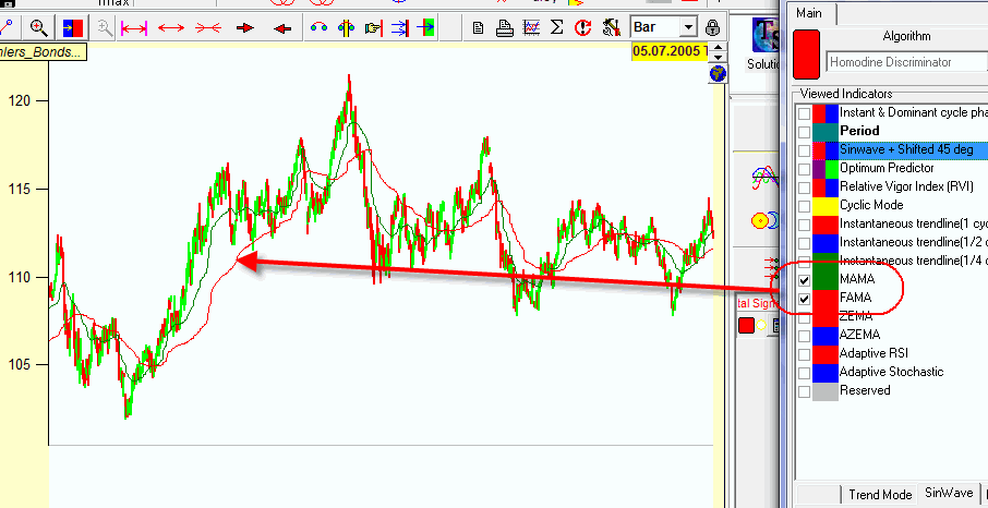
As J.F.Ehlers states "As a result, MAMA and FAMA do not cross unless there has been a major change in the market direction. This suggests an adaptive moving average crossover system that is virtually free of whipsaw trades."
I also recommend to play with "speed" parameter there:
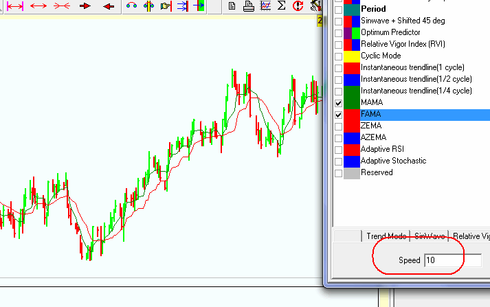
The higher value of the speed parameter, the more fast moving average we have.
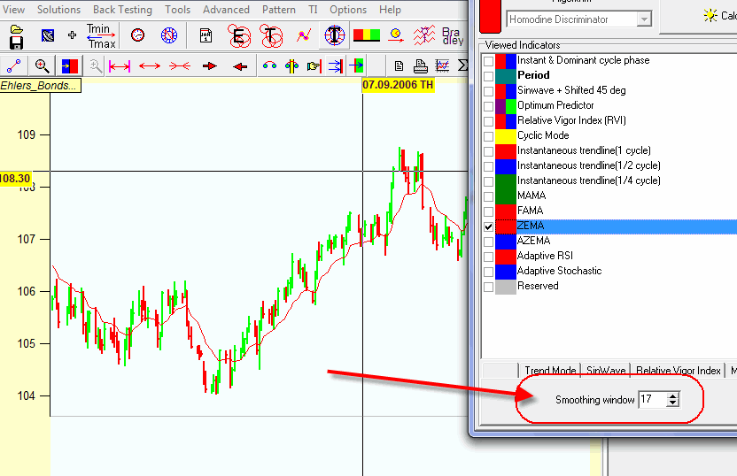
ZEMA (zero lag moving average): this is an adaptive moving average: for the moments when the price changes fast, this moving average changes fast, for slow it changes slow as well. This system assumes the existence of some kind of inertia in the stock market behavior, it assumes that the momentum ( i.e. the speed of the price changes) does not change fast. I recommend to vary the smoothing window for this moving average:
Adaptive RSI and Stochastic - these are standard RSI and Stochastic oscillators though their period is changing while the period of the dominant cycle changes. The rule of their use is exactly the same as the classical rule for standard oscillators. Here the usage of the dominant cycle allows to reveal the cyclic movement more precisely.