Math techniques in Timing Solution

The math methods are especially interesting for me. The reason is that it is simply natural for the person with a solid math background and a working experience of the scientific researcher (20 years at the Institute of Nuclear Research in Russia, http://www.inr.ru). So in this article I describe the math methods presented in Timing Solution. Before going into any discussion, I would like to remind you:

• Timing Solution is not Technical Analysis software. It is developed to generate the projection lines for different financial instruments and verify them. In this regard it is totally different from other tools available on the software market. We believe that the standard approach of Technical Analysis (which is to get buy/sell signals using different combinations of indicators) is very restricted; this is a closed system that tries to get the price from the price itself. We try to model the stock market behavior.
  
• Timing Solution allows to work with huge arrays of data. Having 2GB of RAM on my laptop, I was able to conduct a research for 2.5 millions 1 min price bars (10 years of price history). 
  
• The Back Testing module in Timing Solution is the most powerful module of this kind available on the market. It is a very important part of the program as it is not a big deal to design the projection line that might look very promising; it is much more important to find out how this projection line forecasts when we apply it to another time frame. Back Testing module in Timing Solution is a sample of our ability to solve difficult problems that other software vendors prefer to avoid.
  

All math methods used in Timing Solution can be divided on three groups: 1) descriptive statistics;  2) simple models; 3) Neural Net models with Back Testing module (spectrum, auto regression, wavelets).

Descriptive statistics methods:

These are techniques that any mathematician would perform at first to get a general impression of the analyzed time data set.

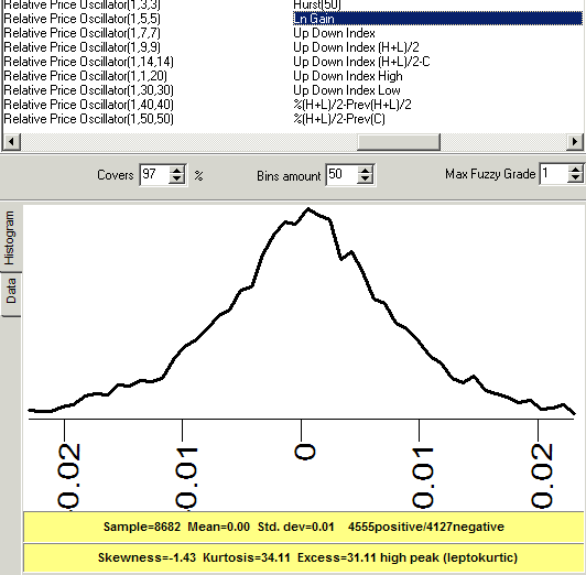
After downloading any price history data, you can immediately look at histograms for different indicators that describe this financial instrument.

This is the histogram for logarithm daily gains calculated for S&P 500 (1974-2008 years):

You can see how B. Mandelbrot's idea of "fat tails" in financial data is confirmed.

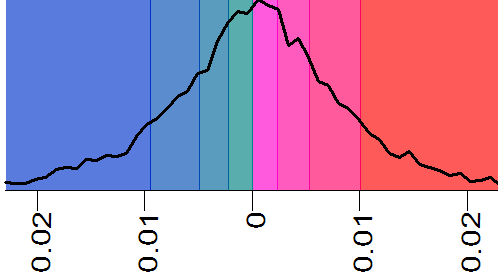
Due to the extensive use of Fuzzy logic methods, you can display these diagrams with weighted zones (all differently colored zones contain the equal amount of points):

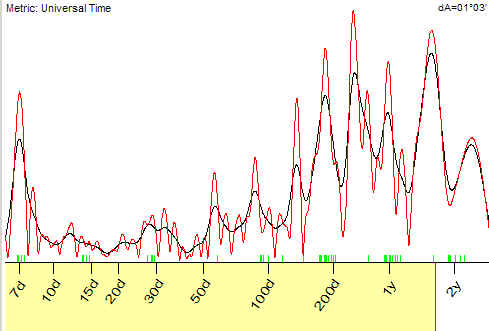
Spectrum analysis. We have spent a lot of time with this module applying the most workable technologies for finance. It took almost 3 years to develop this module, and I can definitely say that for the stock market analysis it is necessary to use totally different approaches than a standard scientific approach.

In general this module allows to reveal the cyclic portrait of any financial instrument. Look at this spectrum calculated for S&P500 index; the relative price oscillator with 100 bars period is used as a target:

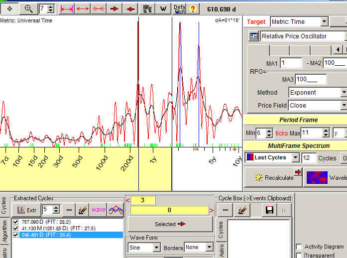
The strongest cycles here are 757 days, 41 months and 246 days.

As a target for spectrum, you can use any other indicator, like volatility,  RSI,  ADX ...

It is a standard procedure of data normalization (detrending) before any spectrum calculations. The most difficult part is finding the algorithms of spectrum calculations suitable for a real stock market. This is the point where our spectrum analysis differs from standard scientific spectrum analysis (which is concentrated mostly on finding the persistent cycles that exist only in an ideal world).

Technically our spectrum module covers three kinds of spectrum: classical, singular spectrum analysis (SSA) and multi scale SSA. The most important thing is that with Timing Solution you can generate projection lines based on the extracted cycle/cycles and conduct back testing for the models used for these projection lines (of course the spectrum is recalculated when new price bars arrive, i.e. we model the real trading).

The technology of creating fast solutions based on spectrum module is described here http://www.timingsolution.com/TS/Study/Classes/class_spectr_1.htm and here http://www.timingsolution.com/TS/Study/Classes/class_spectr_2.htm

Chaos theory module allows to analyze the stock market behavior more deeper. The R/S analysis allows to reveal so called "stochastic cycles":

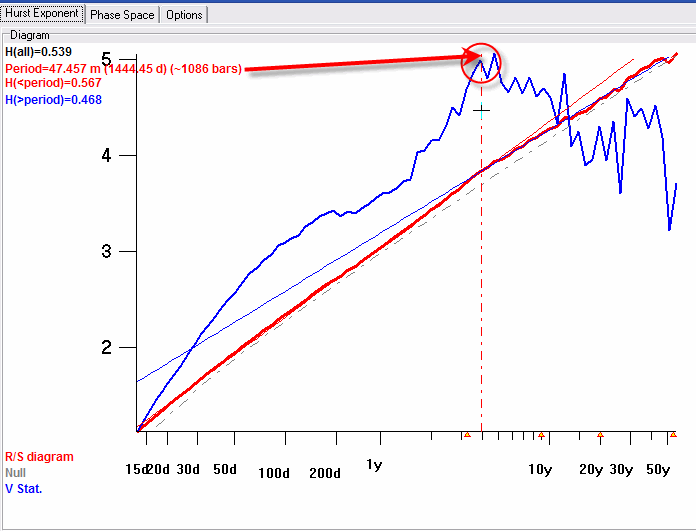
As a target for R/S analysis you can use any indicator. I used daily logarithm gain in the example above.

Here I calculated R/S diagram for Dow Jones Industrial index (data include years 1885-2008). It shows that there is 4 years stochastic cycle, which definitely corresponds to the Presidential cycle. It is impossible to reveal this cycle using spectrum analysis, as the nature of this cycle is different. 

The Chaos Theory module is described here: http://www.timingsolution.com/TS/Articles/Chaos/chaos_ts.htm

Simple models:

These are projection lines created with Annual Cycle module:

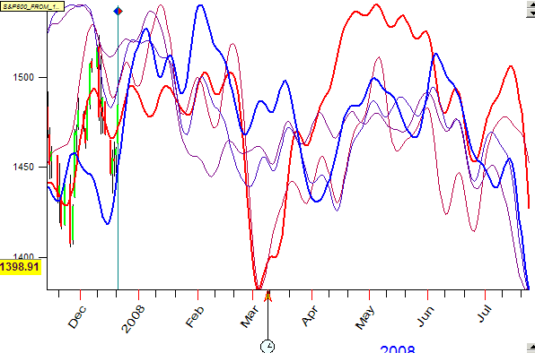
Here five Annual cycles for S&P500 index are shown. The red curve is Annual cycle calculated using the last 2 years of S&P500 history, while to calculate the blue projection line 34 years of price history are used. Thus the blue line points at persistent tendencies in Annual cycle while the red line shows the tendency of the latest 2 years. All other curves represent intermediate variants for Annual cycle.

You can make a forecast based on Fourier analysis just by dragging the mouse from one point to another (say from point A to point B):

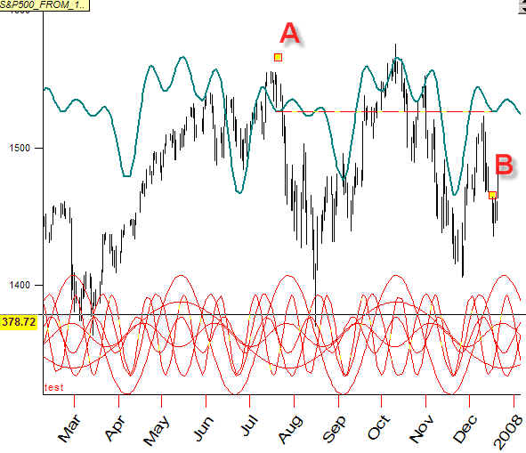
Thus we define the major period for Fourier analysis, and the program automatically performs all other operations of Fourier analysis. It works like a typical charting tool (say Fibonacci retracements or Gann fans).

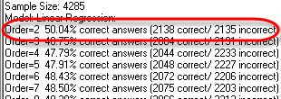
The analysis of Auto regression models can be performed fantastically fast. In the example below, the program has created the Auto regression (AR) model with order 4 (AR4), AR5 ... AR24. See how this AR model forecasts 1 bar ahead (or any other number of bars):

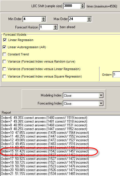
It shows that the best model is AR16. And it took us only several seconds to calculate!

We use this module a lot for artifact studies while conducting the back testing. This is a very important part of back testing procedure.

As an example, let say that somebody claims that he can forecast next day with 80% accuracy, and he forecasts not the price but its moving average. However, it might be not a forecast but some artifact.

So, we calculate that moving average and make a linear regression to forecast the next day moving average value:

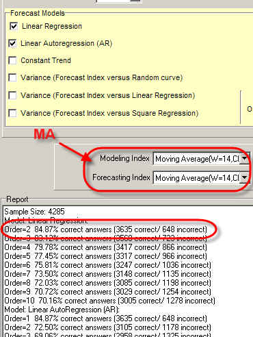
Our result is 85% accurate "forecast". This has happened because the moving average is used as a target for the forecast.

If the same model is applied to forecast "close" instead of moving average, you will get zero:

Neural Network + Back Testing modules:

This combination is the most advanced feature of Timing Solution software. 

Neural Network. The heart of this module is Neural Network (NN). Timing Solution NN allows to generate projection lines based on different models.

These are important features of Timing Solution NN:

• Timing Solution is not Technical Analysis software. The main purpose of this software is generating a projection line of future movement and verifying it. 
  
• We apply the new technology here; it is called Object Oriented Neural Network module. It provides an additional mechanism of optimization besides the standard back propagation. The most important feature of this approach is reducing of over training effect.
  
• We can add easily any event that worth our consideration. For this purpose the special protocol has been developed, we name it Universal Language of Events (ULE). Our Neural Network can work with any event that is described by ULE. Our "know how" is that our Neural Network works not only with digits, it works with events that have many characteristics and reflect some process. The only condition is that the events must be described by ULE. It opens to us the new dimension for optimization. You can find some notes about this technology here: http://www.timingsolution.com/TS/Articles/On_The_Edge/on_the_edge.htm
  
• You can use as many inputs for NN as you need. For some complicated models we use couple thousands of inputs.

As input, you can use:

•  Auto regression (AR) model. Here we use Fuzzy Neural Network technology which is very good to model nonlinear regression models. Some explanation and backtesting results of this approach are here: http://www.timingsolution.com/TS/BT/Candle5/  (this research has been done three years ago; now we provide much more detailed backtesting).
  The AR model can involve more than hundreds of different indicators, using any order of regression.
  
• Cycles extracted by Spectrum module (the program calculates spectrum, extracts from it %X the most powerful cycles and generates the projection line based on these cycles).
  
• Wavelet model.

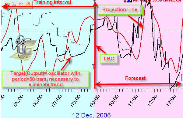
Back Testing Module. If the projection line can be calculated by Neural Network module, we can provide a detailed back testing for this model. The program divides the whole price history file on two intervals. One interval is used to calculate spectrum (if this is spectrum model) and train Neural Network. The other interval ("out of sample") serves to check how this model forecasts the future. The program performs this procedure as many times as you need.

The program excludes any kind of "future leaks", in other words there will be no surprises (like the model that earlier has worked perfectly does not work at all now).

For example the back testing process for Spectrum based model can be something like this:

a) Break the price history on training and testing intervals

b) Calculate the Spectrum diagram using price history from the training interval:

c) Extract the most important cycles from this spectrum:

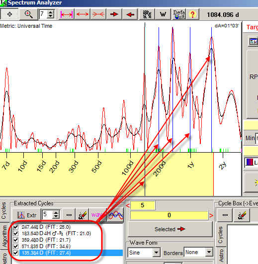
d) Use these cycles as inputs for Neural Network module and generate the projection line based on these cycles:

e) Check how the program forecasts on TESTING interval (there are many criteria like calculate a correlation between the price and the projection line, %X trades based on turning points created by the projection line, or the direction of future movement).

f) The program repeats this procedure using other training and testing intervals and repeats this procedure again (recalculates spectrum, creates a new Neural Net, etc.).

Some info regarding Back Testing procedure you can find here: http://www.timingsolution.com/TS/Study/BT/

If you need to get the list of the projection lines generated by different techniques, you can get a report similar to these ones:

for autoregressoion model: ar.pdf

for spectrum model: spectr.pdf

To make backtesting procedure statistically significant, usually we analyze hundreds of projection lines.

The special issue is artifact study within backtesting procedure. This is a very tricky and time consuming process. We spent 3 hard working years to reveal all (I hope) artifact effects common to forecasting.